Prof D’s Regression Sessions - Vol 2
Time to go even deeper!
Adam Dennett - a.dennett@ucl.ac.uk
2025-26
CASA0007 Quantitative Methods
This week’s Session Aims
- Build on the basics you learned last week and learn how to extend regression modelling into multiple dimensions
- Understand the main benefits, risks and steps to take when gradually building the complexity of your models
- Understand who to interpret the outputs correctly
- Gain an appreciation of how regression help explain the phenomena we are observing
- Have hands-on practice at building and interpreting your own complex models
Recap - Last Week’s Model
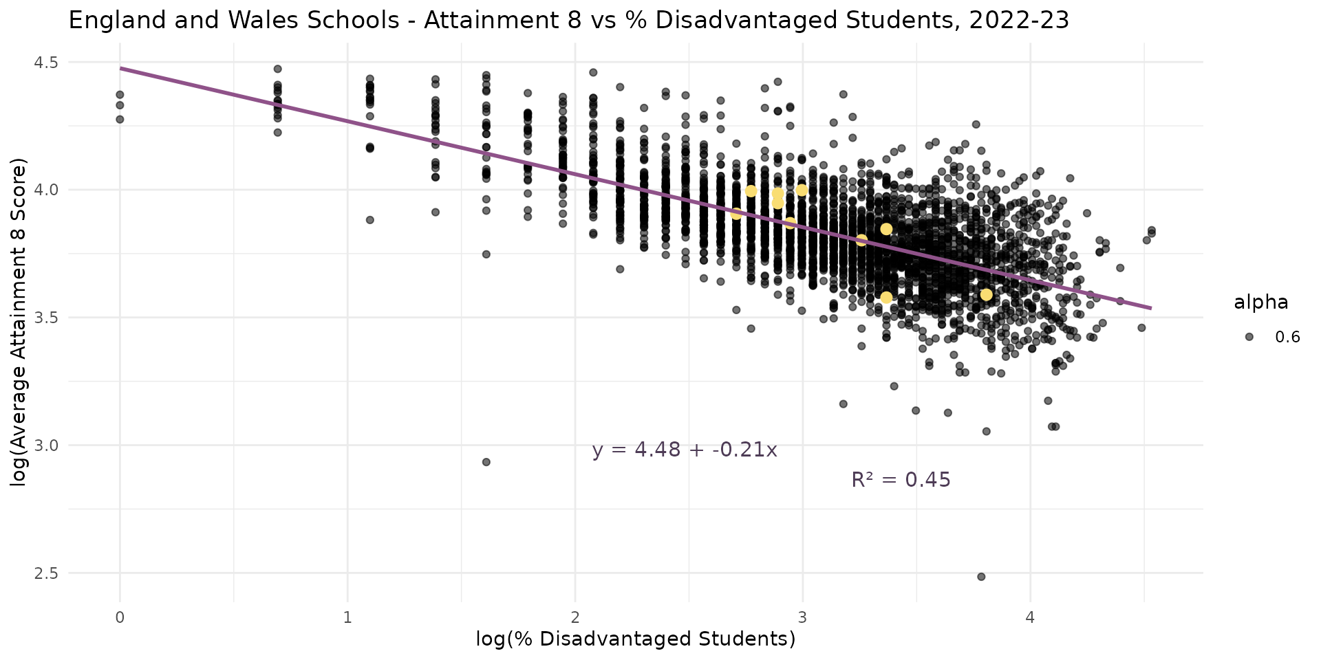
- Work of Gorard suggested link between levels of disadvantage in a school and attainment.
- Not a linear relationship but a log-log elasticity
Recap - Last Week’s Model
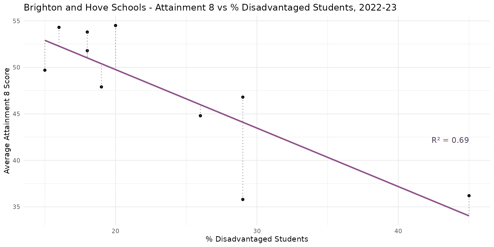
- School-level relationship between attainment and disadvantage unreliable at the local authority level with small changes influencing coefficients where degrees of freedom are low
An Alternative Model
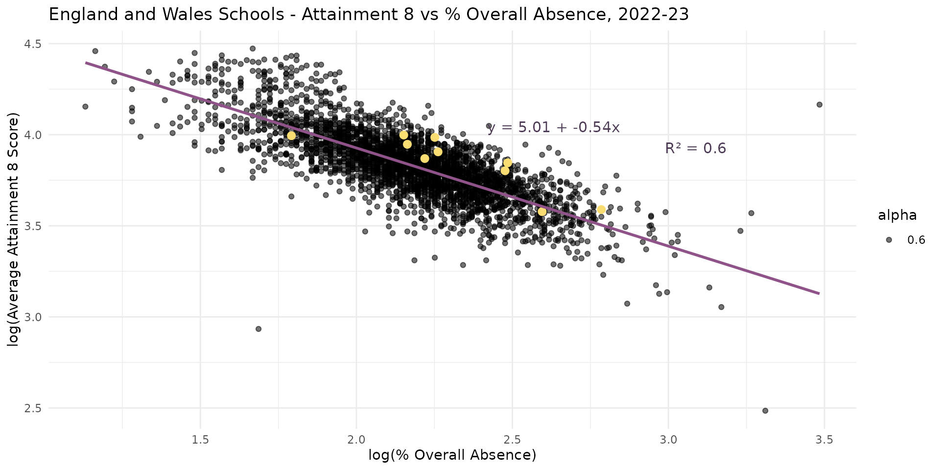
- Other research suggests overall levels of absence might be even more important
- How can we tell for sure?
An Alternative Model
Call:
lm(formula = log(ATT8SCR) ~ log(PERCTOT), data = england_filtered)

Residuals:
     Min       1Q   Median       3Q      Max
-1.16241 -0.07336  0.00471  0.07247  1.03789

Coefficients:
             Estimate Std. Error t value Pr(>|t|)
(Intercept)   5.00521    0.01712  292.40   <2e-16 ***
log(PERCTOT) -0.53898    0.00778  -69.27   <2e-16 ***
---
Signif. codes:  0 '***' 0.001 '**' 0.01 '*' 0.05 '.' 0.1 ' ' 1

Residual standard error: 0.1223 on 3231 degrees of freedom
  (15 observations deleted due to missingness)
Multiple R-squared:  0.5976,    Adjusted R-squared:  0.5975
F-statistic: 4799 on 1 and 3231 DF, p-value: < 2.2e-16- Overall Absence = bigger coefficient (-0.54 vs -0.21) & improves the \(R^2\) to (60% vs 45% for the % disadvantage model)
- Suggests that Overall Absence explains more variation in Attainment 8
Multiple Linear Regression
- One way to really tell which variable is more important is to put them in a model together and observe how the affect each other
- Multiple linear regression extends bivariate regression to include multiple independent variables
- As with bivariate regression, variables should be chosen based on theory and prior research rather than just throwing the variables in because you have them
- However, it’s permissible to explore relationships and experiment and iterate between data exploration and theory - both can inform each other
Multiple Linear Regression
- When we start adding more variables into the model, an alternative to the more generic notation is to include the variables in the equation explicitly, for example:
\[\log(\text{Attainment8}) = \beta_0 + \beta_1\log(\text{PctDisadvantage}) +\\\\ \beta_2log(\text{PctOverallAbsence}) + \epsilon\]
- There’s no real limit to the number of variables you can include in a model - however:
- Fewer is easier to interpret
- More variables will reduce your degrees of freedom
Multiple Linear Regression
Multiple Linear Regression
Call:
lm(formula = log(ATT8SCR) ~ log(PTFSM6CLA1A) + log(PERCTOT),
    data = model_data)

Residuals:
     Min       1Q   Median       3Q      Max
-1.26481 -0.06531 -0.00040  0.06352  0.77403

Coefficients:
                  Estimate Std. Error t value Pr(>|t|)
(Intercept)       5.063088   0.015126  334.72   <2e-16 ***
log(PTFSM6CLA1A) -0.111473   0.003578  -31.16   <2e-16 ***
log(PERCTOT)     -0.406199   0.008045  -50.49   <2e-16 ***
---
Signif. codes:  0 '***' 0.001 '**' 0.01 '*' 0.05 '.' 0.1 ' ' 1

Residual standard error: 0.1072 on 3230 degrees of freedom
Multiple R-squared:  0.6906,    Adjusted R-squared:  0.6904
F-statistic: 3605 on 2 and 3230 DF, p-value: < 2.2e-16- What is the model telling us?
Multiple Linear Regression
| AIC | AICc | BIC | R2 | R2 (adj.) | RMSE | Sigma |
|---|---|---|---|---|---|---|
| 19500.8 | 19500.8 | 19525.1 | 0.69 | 0.69 | 0.11 | 0.11 |
Multiple Linear Regression
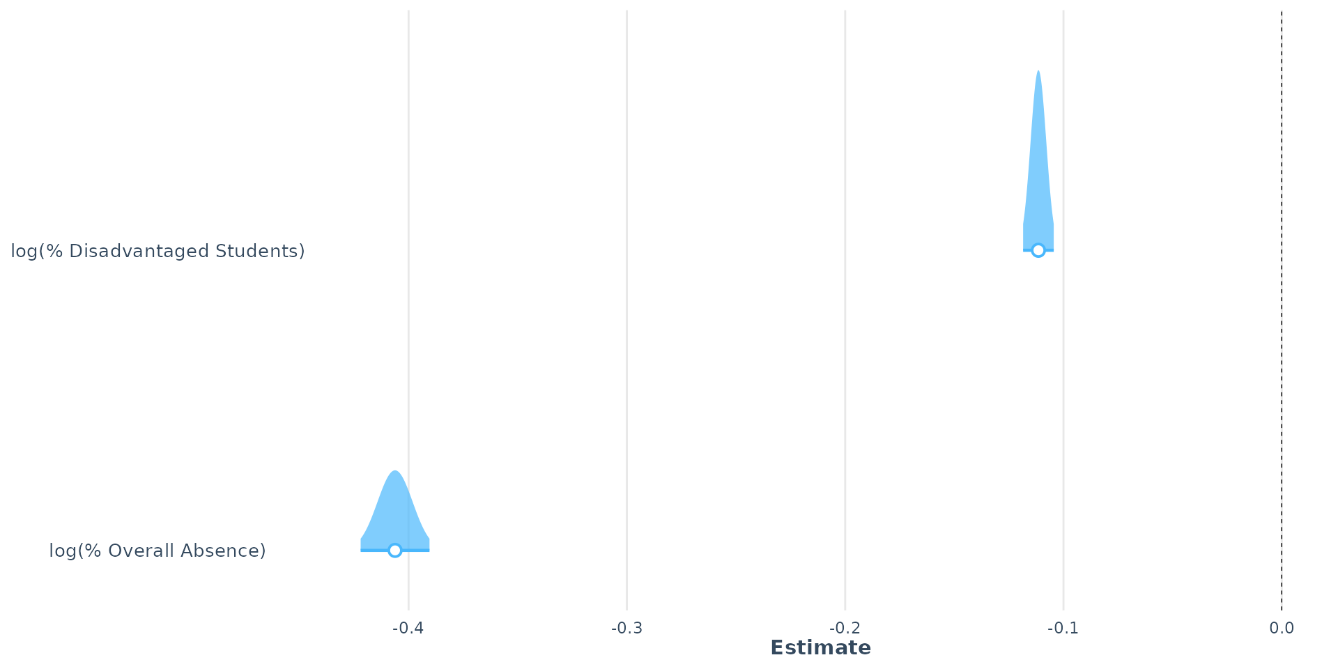
- The coefficients for both variables are statistically significant and negative, indicating that both variables contribute to explaining the variation in Attainment 8 scores
- The t-values suggest the % Overall Absence variable (-50.49) is doing more work than the % Disadvantaged Students variable (-31.16) - but hold that thought, because ranking predictors this way is harder than it looks and we come back to it after the diagnostics
- The \(R^2\) value is now 0.69, indicating that the model is potentially good and explains 69% of the variation in Attainment 8 scores. Degrees of freedom are good and the overall model is statistically significant.
- But does it satisfy the assumptions of linear regression?
Diagnostics 1
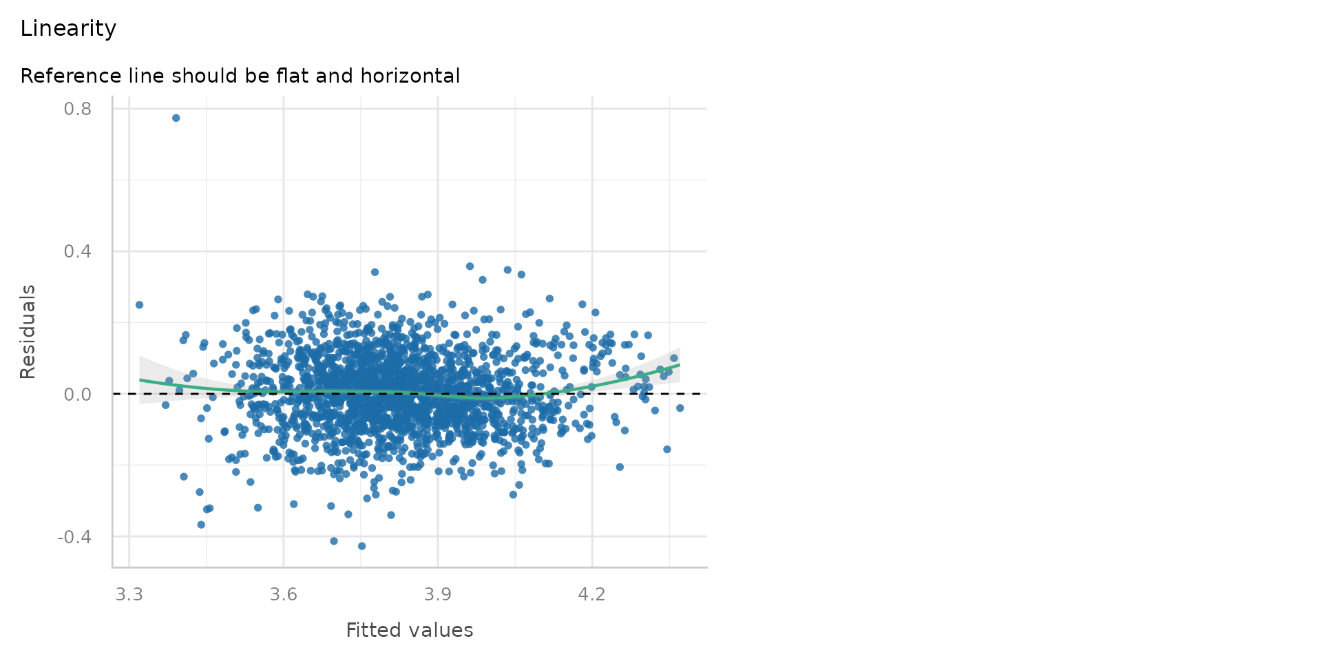
- Pretty good - the residuals are randomly scattered around zero, suggesting a linear relationship
Diagnostics 2
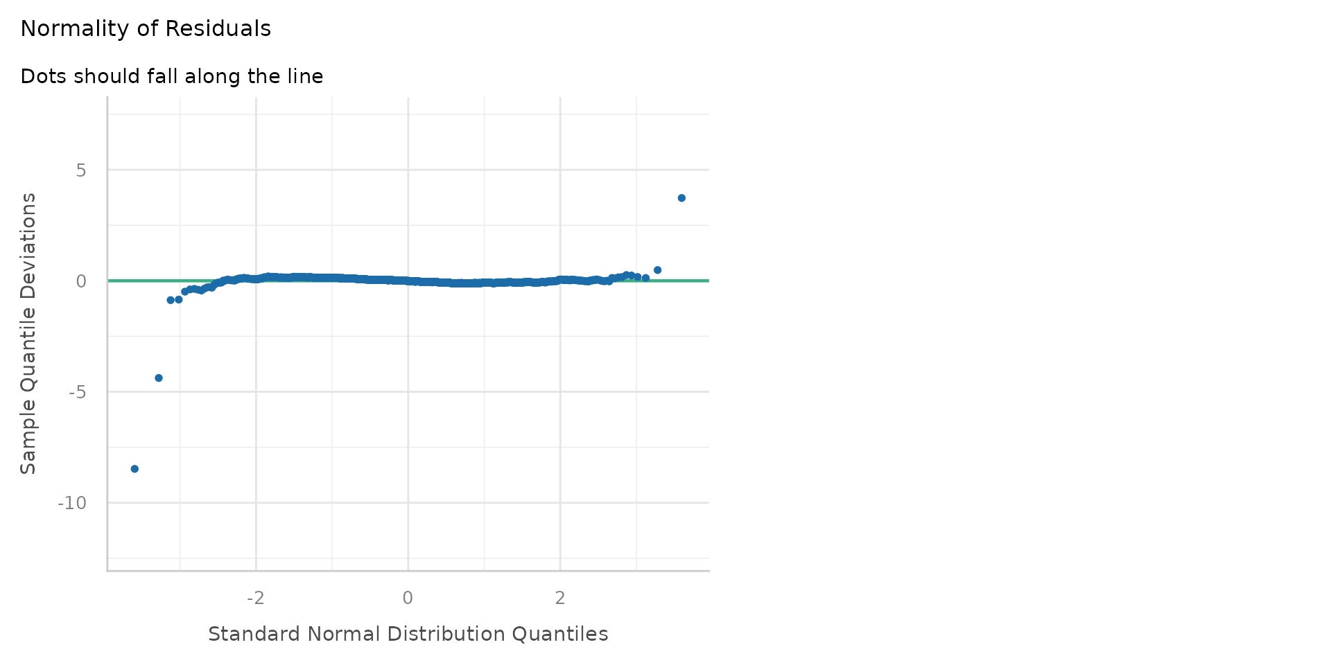
- The residuals are normally distributed - the Q-Q plot shows most points on the line
Diagnostics 3
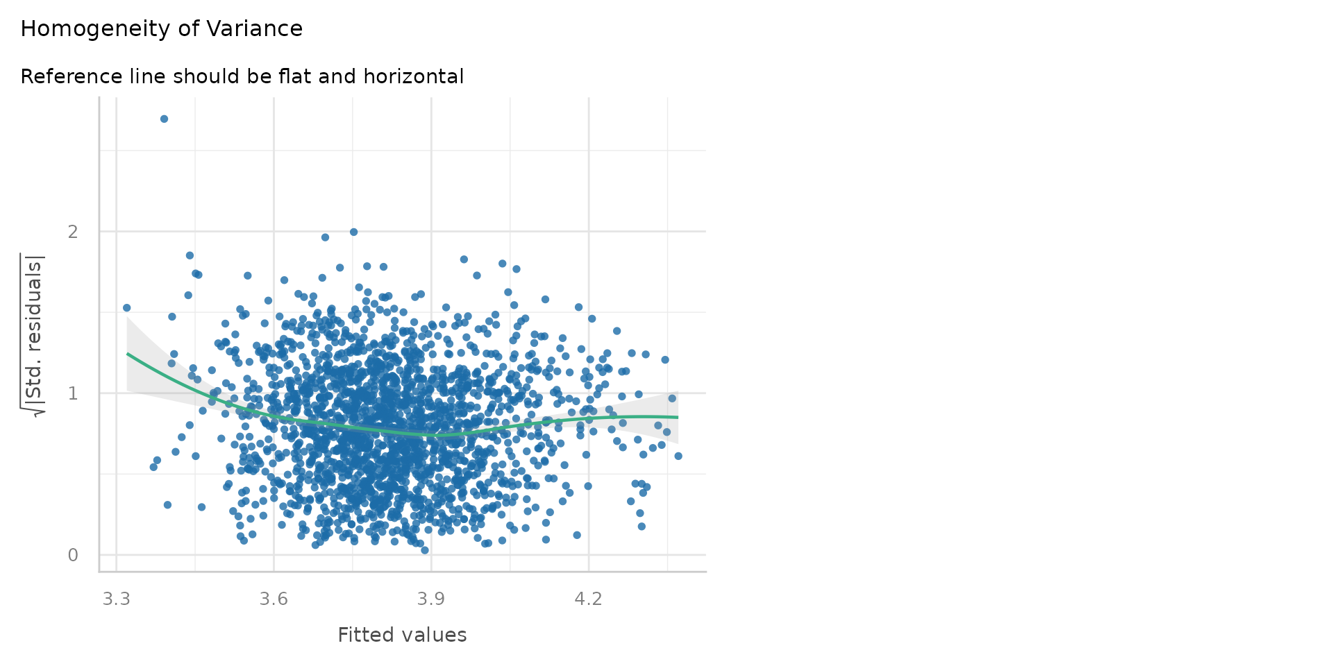
- The residuals are randomly scattered around zero, suggesting constant variance.
Linear Regression - Diagnostics
- Linearity: 😎
- Homoscedasticity: 😎
- Normality of residuals: 😎
- No multicollinearity: 😕
- Independence of residuals: 😕
Multicollinearity
- Multicollinearity occurs when two or more independent variables in a regression model are highly correlated with each other
- This can lead to unreliable estimates of the coefficients, inflated standard errors, and difficulty in interpreting the results
Multicollinearity
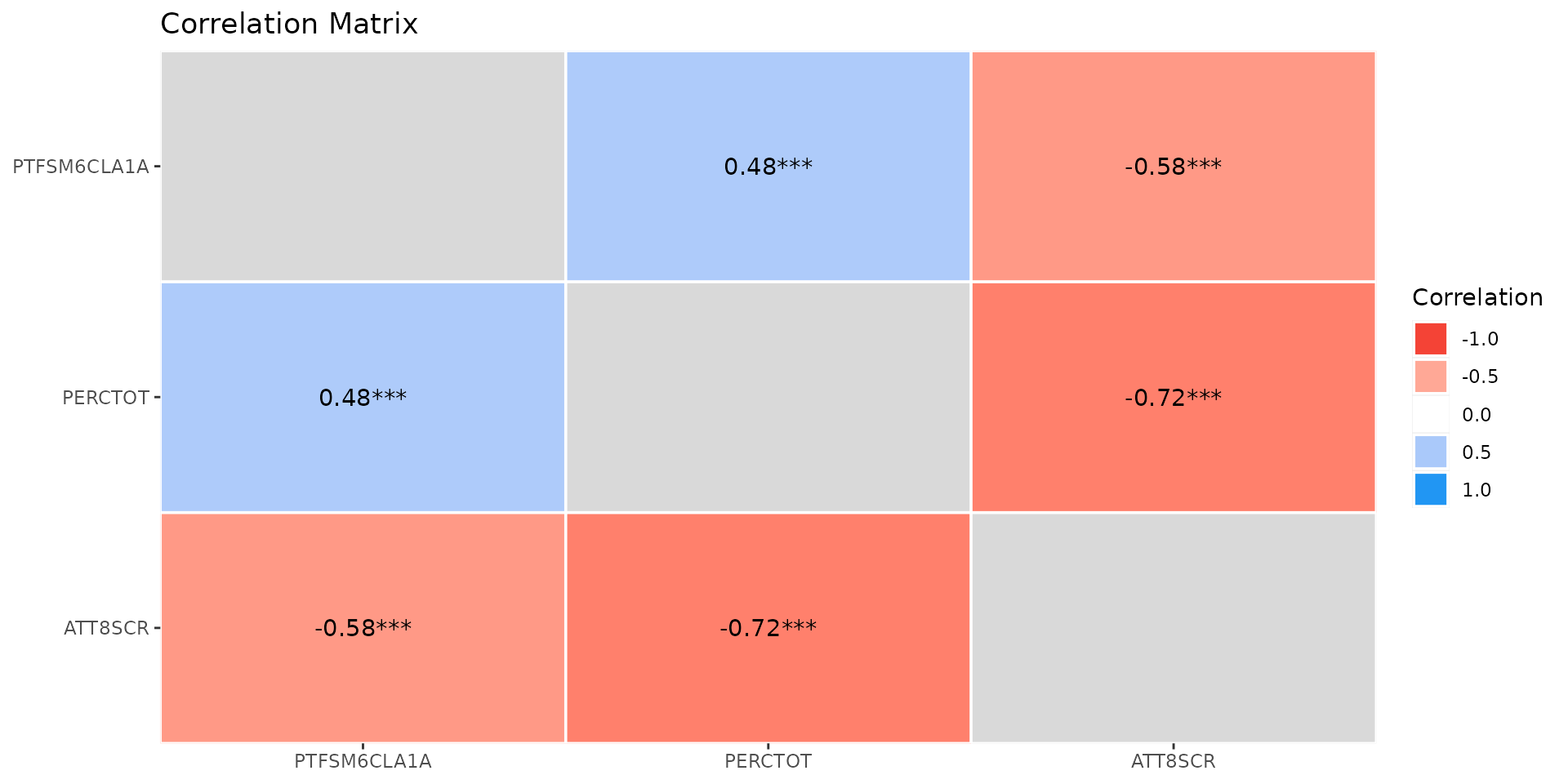
- A quick and easy way to check for the correlation between your independent variables is generate a standard correlation matrix/plot
- Difficult to say what is too much correlation - but over 0.7 is often considered problematic
- However, pairwise correlations might miss n-way correlations
Variance Inflation Factor - VIF
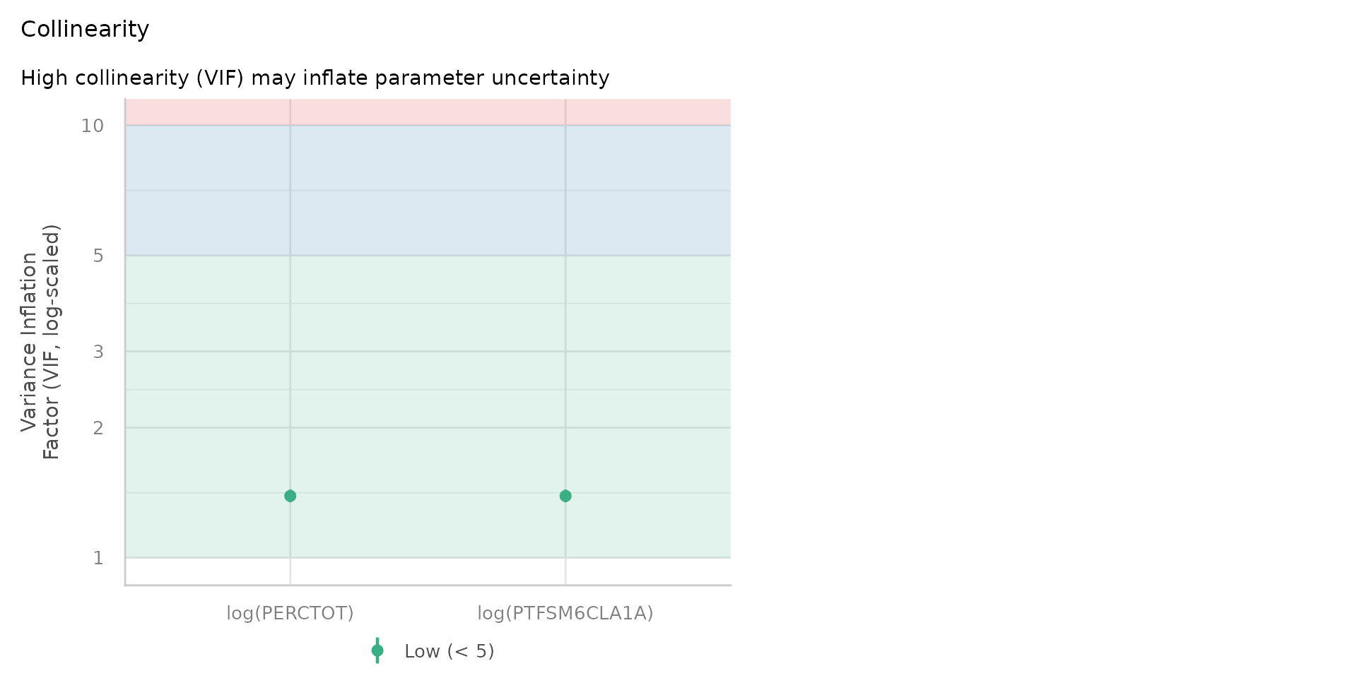
- A more useful diagnostic tool is the Variance Inflation Factor (VIF), which measures how much the variance of a regression coefficient is increased due to multicollinearity
- A VIF value of 1 indicates no correlation, while a VIF value above 5 or 10 suggests high multicollinearity
Variance Inflation Factor - VIF
Why does it even matter if the variance is inflated?
- Variance = Uncertainty in our model
- If 2 or more variables are highly correlated and both appear to affect the dependent variable, it can be difficult to determine which variable is actually having the effect
- The model makes an arbitrary split
- Small changes in the data could make the split go either way - e.g. attribute more of the effect to % Disadvantaged Students or % Overall Absence (if VIF high) - thus inflating the uncertainty / variance
Variance Inflation Factor - VIF
- Despite some positive correlation (0.48) between % Disadvantaged Students and % Overall Absence, the VIF is very low ~1.5
- No problems with multicollinearity
- So we have passed that test and can happily use both in the model
So which variable actually matters more?
- Earlier we said the t-values made % Overall Absence look like the stronger predictor. That comparison is shakier than it appears.
- A t-value is \(\frac{\text{Estimate}}{\text{SE}}\), so it mixes up how big an effect is with how precisely we have measured it
- With 3,233 schools, everything is precisely measured, so the t-values mostly tell us about sample size
- And there is a deeper problem - one we have already met under a different name
The two variables overlap
| \(R^2\) | |
|---|---|
| % Disadvantaged on its own | 0.446 |
| % Overall Absence on its own | 0.598 |
| Both together | 0.691 |
| Sum of the two separately | 1.044 |
- The two on their own add up to 1.044, but together they explain only 0.691
- The difference - 0.353 - is variance the two variables share. It is explained by either of them, and owned by neither
- That is 51% of everything the model explains. This is the VIF problem again: the model has to make an arbitrary split, and the t-values inherit it
Shapley values - splitting the shared variance fairly
- Instead of letting the model split the shared variance arbitrarily, we can average over every possible order in which the variables could enter
- Add disadvantage first, then absence. Then absence first, then disadvantage. Average what each one gained
- This is the Shapley value, known in regression as the LMG decomposition
r2_of <- function(vs) {# R² of a model with these variables
  rhs <- if (length(vs) == 0) "1" else paste(vs, collapse = " + ")
  summary(lm(as.formula(paste("log(ATT8SCR) ~", rhs)), data = decomp_data))$r.squared
}

# average each variable's gain across both orders of entry
shap["fsm"] <- mean(c(r2_of("fsm"), r2_of(c("abs","fsm")) - r2_of("abs")))
shap["abs"] <- mean(c(r2_of(c("fsm","abs")) - r2_of("fsm"), r2_of("abs")))
In R, relaimpo::calc.relimp(model, type = "lmg") does this for you. Shapley (1953); Lindeman, Merenda & Gold (1980); Grömping (2007) The American Statistician 61(2) 139-147
What the decomposition says
| Shapley \(R^2\) | Share of explained | |
|---|---|---|
| % Disadvantaged | 0.270 | 39.1% |
| % Overall Absence | 0.421 | 60.9% |
| Total | 0.691 | 100% |
- The shares sum exactly to the model’s \(R^2\) (0.691) - nothing is lost or double-counted
- Absence takes 61% of the explanation, disadvantage 39%
- Here the ranking happens to agree with the t-values - but now it is a defensible number rather than a side-effect of sample size, and we also know that 51% of the explanation is shared between the two
- Two warnings: a Shapley share has no sign (it cannot tell you whether an effect is positive or negative), so always report it alongside the coefficients - and the cost grows as \(2^k\), so it gets slow with many predictors
Linear Regression - Diagnostics
- Linearity: 😎
- Homoscedasticity: 😎
- Normality of residuals: 😎
- No multicollinearity: 😎
- Independence of residuals: 😕
Independence of Residuals
- Residuals (errors) should not be correlated with each other
- (auto)correlation (clustering) in the errors = model missing something!
- can lead to biased estimates and incorrect conclusions
- often occurs when a temporal or spatial component to the data
- or when another important variable is missing or omitted
Spatial or Temporal (auto)Correlation
- In our case, we have a spatial component to the data - schools are located in different areas of England and Wales
- If schools in the same area have similar characteristics, it is likely that the residuals will be correlated
- The easiest way to check this is to plot the values of the residuals for the schools on a map
Residual (auto)Correlation
- Residuals show clear spatial autocorrelation
- London (and other city schools) perform much better than model predicts
Residual (auto)Correlation
- ALWAYS MAP YOUR RESIDUALS IF MODELLING SPATIAL DATA
- Correlated residuals often the sign of an omitted variable (e.g “London”)
- In the GIS Course you will learn a lot more about testing for spatial autocorrelation (using Moran’s I) and how spatial variables (lags, error terms) or geographically weighted regression can be used to deal with spatial autocorrelation
- Here we will try something much simpler - adding London (and other regions) to our model
Linear Regression - Diagnostics
- Linearity: 😎
- Homoscedasticity: 😎
- Normality of residuals: 😎
- No multicollinearity: 😎
- Independence of residuals: 😬
Dummy Variables
Dummy Variables
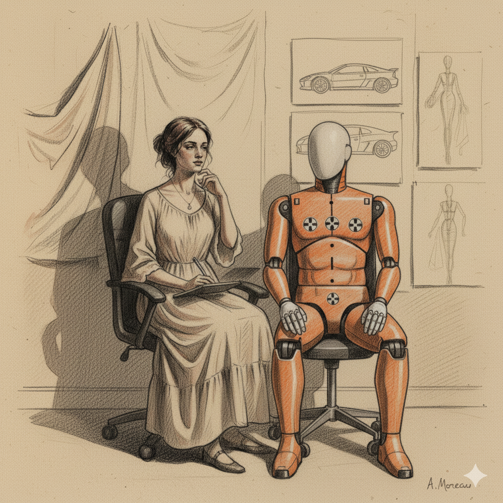
- In linear regression, independent variables can also be categorical
- Categorical variables are often referred to as DUMMY variables
- Dummy because the are a numerical stand-in (1 or 0) for a qualitative concept
- In our model Region could be a dummy variable to see the “London” effect is real
- Dummy could also be any other categorical variable like Ofsted rating (e.g. Good, Outstanding etc.)
Dummy Variables
Call:
lm(formula = log(ATT8SCR) ~ log(PTFSM6CLA1A) + log(PERCTOT) +
    gor_name, data = model_data)

Residuals:
     Min       1Q   Median       3Q      Max
-1.24928 -0.05827  0.00088  0.06062  0.73259

Coefficients:
                                  Estimate Std. Error t value Pr(>|t|)
(Intercept)                       5.010071   0.015920 314.710  < 2e-16 ***
log(PTFSM6CLA1A)                 -0.132708   0.003801 -34.910  < 2e-16 ***
log(PERCTOT)                     -0.366326   0.008373 -43.752  < 2e-16 ***
gor_nameEast of England           0.006536   0.008173   0.800 0.423949
gor_nameLondon                    0.100077   0.007890  12.683  < 2e-16 ***
gor_nameNorth East                0.079556   0.010500   7.577 4.61e-14 ***
gor_nameNorth West                0.008348   0.007786   1.072 0.283680
gor_nameSouth East                0.004422   0.007724   0.573 0.566995
gor_nameSouth West                0.031877   0.008486   3.757 0.000175 ***
gor_nameWest Midlands             0.033315   0.008067   4.130 3.72e-05 ***
gor_nameYorkshire and the Humber  0.040358   0.008426   4.789 1.75e-06 ***
---
Signif. codes:  0 '***' 0.001 '**' 0.01 '*' 0.05 '.' 0.1 ' ' 1

Residual standard error: 0.1025 on 3222 degrees of freedom
Multiple R-squared:  0.7182,    Adjusted R-squared:  0.7173
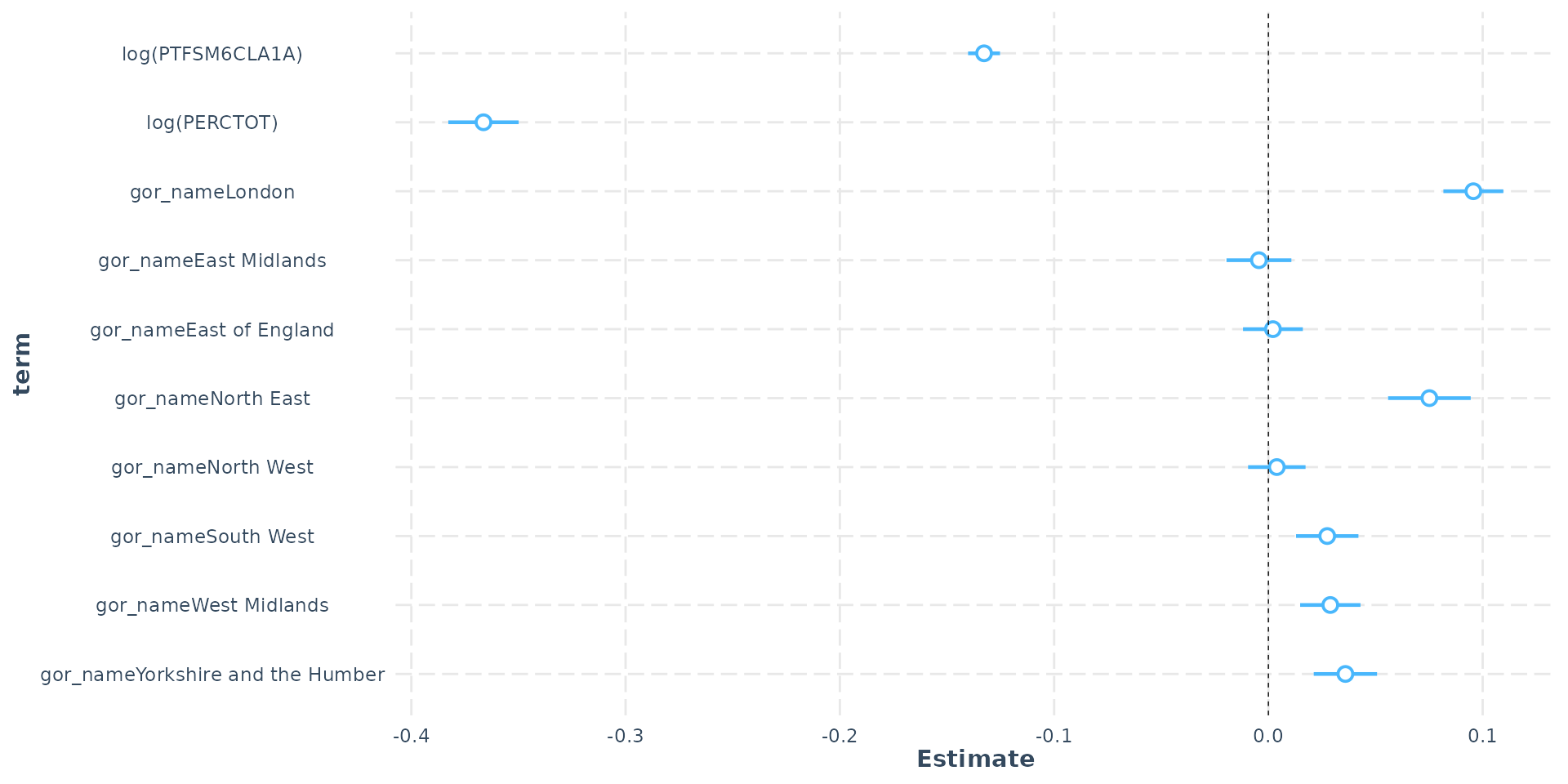
F-statistic: 821 on 10 and 3222 DF, p-value: < 2.2e-16- There are 9 regions in England and here “London” has been set as the contrast or reference variable (which all others are compared to)
- Changing the contrast compares each region to a different reference
Dummy Variables
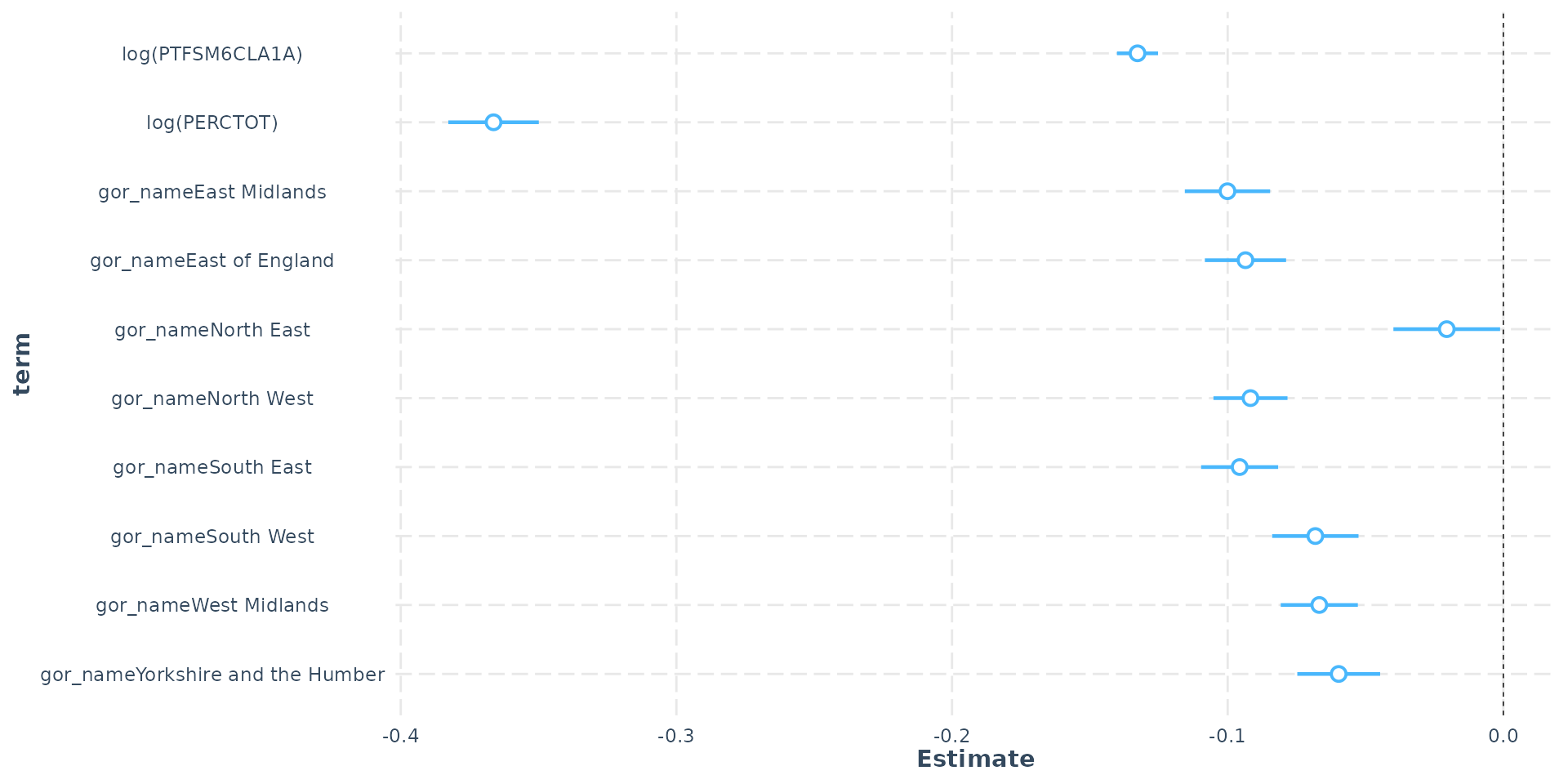
- Government Office Region (GOR) dummy - (London as ref)
Dummy Variables
Call:
lm(formula = log(ATT8SCR) ~ log(PTFSM6CLA1A) + log(PERCTOT) +
    gor_name, data = model_data)

Residuals:
     Min       1Q   Median       3Q      Max
-1.24928 -0.05827  0.00088  0.06062  0.73259

Coefficients:
                                  Estimate Std. Error t value Pr(>|t|)
(Intercept)                       5.014493   0.015398 325.660  < 2e-16 ***
log(PTFSM6CLA1A)                 -0.132708   0.003801 -34.910  < 2e-16 ***
log(PERCTOT)                     -0.366326   0.008373 -43.752  < 2e-16 ***
gor_nameLondon                    0.095655   0.007131  13.413  < 2e-16 ***
gor_nameEast Midlands            -0.004422   0.007724  -0.573 0.566995
gor_nameEast of England           0.002114   0.007119   0.297 0.766538
gor_nameNorth East                0.075134   0.009836   7.638 2.88e-14 ***
gor_nameNorth West                0.003926   0.006840   0.574 0.566020
gor_nameSouth West                0.027455   0.007428   3.696 0.000223 ***
gor_nameWest Midlands             0.028893   0.007181   4.023 5.87e-05 ***
gor_nameYorkshire and the Humber  0.035935   0.007533   4.770 1.92e-06 ***
---
Signif. codes:  0 '***' 0.001 '**' 0.01 '*' 0.05 '.' 0.1 ' ' 1

Residual standard error: 0.1025 on 3222 degrees of freedom
Multiple R-squared:  0.7182,    Adjusted R-squared:  0.7173
F-statistic: 821 on 10 and 3222 DF, p-value: < 2.2e-16- South East as contrast - London’s log(ATT8SCR) is 0.09 higher
- This equals (exp(0.095655) - 1) * 100 = 10% - London’s average Attainment 8 is 10% higher than the South East
Dummy Variables
Dummy Variables
- Hard to tell definitively from visual map, but residuals have changed and less clustering (Moran’s I would be more definitive - see GIS course)
Dummy Variables
- There is no correct contrast to choose for your dummy variable, you may need to try different ones to see which makes most intuitive sense
- Depending on the contrast, some dummy regions may or may not be statistically significant in comparison
- The inclusion of a regional dummy in this model has improved the \(R^2\) to 72%
- However, you may have noticed some of the coefficients have changed and this brings us to confounding and mediation
Variable Reclassification
A Quick Aside:
- One potentially useful strategy in regression modelling is the reclassification of an independent variable.
- Continuous -> Categorical or Weak Ordinal (e.g. various measurements of height into short, average and tall at different thresholds)
- Categorical -> Categorical with fewer categories (e.g. short, average, tall into below average and above average)
Variable Reclassification
- Benefits of reclassification:
- Moving from a continuous variable to a weak ordinal variable might make the patterns or observations easier to explain
- complex relationships (such as log-linear elasticities associated with absence from school) reduced to something more interpretable (if you miss more than 50% of school, your odds of passing your exams are drastically reduced)
- Previous obscured patterns can emerge from the data
- Collapsing categorical variables (e.g. multiple religious school denominations into religious/non-religious) can aid interpretability and boost statistical power, increase degrees of freedom
Variable Reclassification
- Risks of reclassification:
- Loss of statistical power due to loss of information
- Not always obvious where to make the cut when reclassifying a continuous variable and this can be crucial to the interpretation (e.g. is Low <20 or <30?)
Confounding

Confound: “to fail to discern differences between : mix up”
Confounding
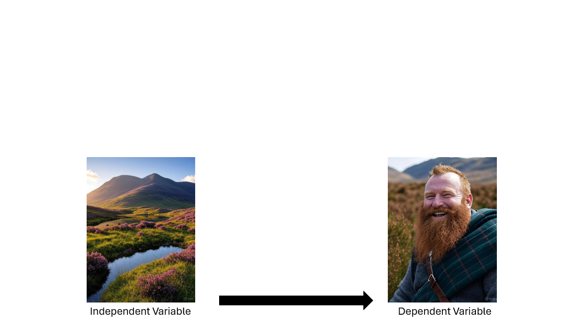
Confounding
Confounding
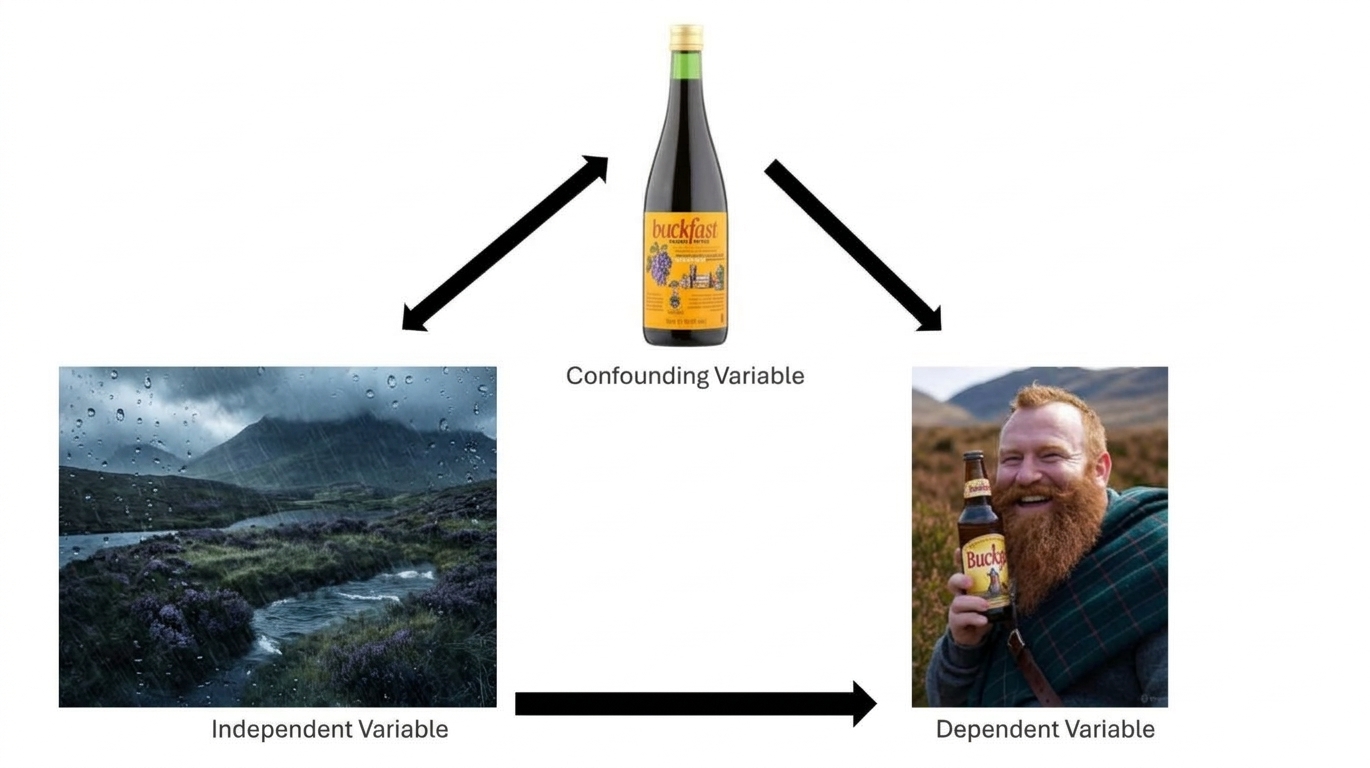
- Look at the arrows in that picture. The confounder is not sitting between the two variables - it is sitting above both of them, with an arrow running down to each
- That is what makes something a confounder: it is a common cause. It causes the independent variable and it causes the dependent variable
- The result is that \(X\) and \(Y\) move together without \(X\) doing anything to \(Y\). Some - or all - of the association you can see is really the confounder showing through both of them
- Drop the confounder into the model and that borrowed association is handed back to its owner, so the coefficient on \(X\) changes
- In the picture: the Buckfast makes the rainy glen (\(X\)) look glorious, and it makes the man (\(Y\)) happy. Glen and mood move together - but the glen is not what is cheering him up. Take the Buckfast away and the association goes with it
Confounding
- So in practice you spot confounding by its symptom: the effect of one independent variable changes in the presence of another
- This can happen even when the two are not correlated enough to cause any variance problems - confounding and multicollinearity are different things
- Looking for confounding effects is a crucial part of model building - how do the coefficients of your model change when you introduce other variables?
- But a word of warning, which we will come back to after mediation: a coefficient changing is the symptom of more than one underlying structure
Confounding
| Model 1 | Model 2 | Model 3 | |
|---|---|---|---|
| (Intercept) | 4.48 *** | 5.01 *** | 5.06 *** |
| log(PTFSM6CLA1A) | -0.21 *** | -0.11 *** | |
| log(PERCTOT) | -0.54 *** | -0.41 *** | |
| N | 3248 | 3233 | 3233 |
| R2 | 0.45 | 0.60 | 0.69 |
| *** p < 0.001; ** p < 0.01; * p < 0.05. | |||
- Disadvantage is the common cause here. Poverty makes it harder to get to school - so it drives absence - and it depresses attainment by other routes entirely: family support, resources, housing, health
- So when we ask “what is the effect of absence on attainment?”, disadvantage is a confounder. Part of what looks like absence doing the work is really disadvantage showing through both
- Which is exactly why the absence coefficient shrinks once disadvantage joins the model
- Both variables together explain much more variation in Attainment 8 - both are part of the story
Confounding
Confounding
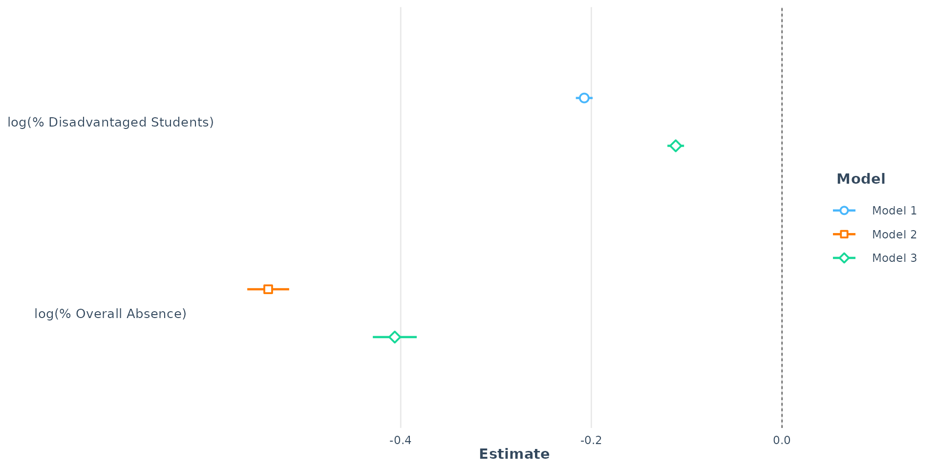
- Disadvantage - log(PTFSM6CLA1A) - shrinks dramatically, from -0.21 to -0.11, a 44.5% reduction
- Overall Absence - log(PERCTOT) - shrinks from -0.54 to -0.41, just 24.6%
- The two shrinkages are not the same kind of thing, because the causal arrows do not run both ways:
- Absence shrinks because disadvantage was confounding it - some of what looked like absence was poverty showing through
- Disadvantage shrinks more because absence is carrying part of disadvantage’s own effect - that is mediation, not bias
- Resist the urge to call either one the “right” answer. Which you want depends on what you are asking - and we settle that after mediation
Confounding
Call:
lm(formula = log(ATT8SCR) ~ log(PTFSM6CLA1A) + log(PERCTOT) +
    gor_name, data = model_data)

Residuals:
     Min       1Q   Median       3Q      Max
-1.24928 -0.05827  0.00088  0.06062  0.73259

Coefficients:
                                  Estimate Std. Error t value Pr(>|t|)
(Intercept)                       5.014493   0.015398 325.660  < 2e-16 ***
log(PTFSM6CLA1A)                 -0.132708   0.003801 -34.910  < 2e-16 ***
log(PERCTOT)                     -0.366326   0.008373 -43.752  < 2e-16 ***
gor_nameLondon                    0.095655   0.007131  13.413  < 2e-16 ***
gor_nameEast Midlands            -0.004422   0.007724  -0.573 0.566995
gor_nameEast of England           0.002114   0.007119   0.297 0.766538
gor_nameNorth East                0.075134   0.009836   7.638 2.88e-14 ***
gor_nameNorth West                0.003926   0.006840   0.574 0.566020
gor_nameSouth West                0.027455   0.007428   3.696 0.000223 ***
gor_nameWest Midlands             0.028893   0.007181   4.023 5.87e-05 ***
gor_nameYorkshire and the Humber  0.035935   0.007533   4.770 1.92e-06 ***
---
Signif. codes:  0 '***' 0.001 '**' 0.01 '*' 0.05 '.' 0.1 ' ' 1

Residual standard error: 0.1025 on 3222 degrees of freedom
Multiple R-squared:  0.7182,    Adjusted R-squared:  0.7173
F-statistic: 821 on 10 and 3222 DF, p-value: < 2.2e-16- Including a regional dummy slightly reduces the effect of Overall Absence and slightly increases the effect of disadvantage, relative to model 3
Confounding
Interpretation:
- Part of the negative effect of disadvantage was being suppressed or masked by the regional differences (probably London where Attainment 8 is higher on average and so are levels of disadvantage)
- Part of the negative effect of Overall Absence is due to its correlation with regional factors - but which ones?
- We can explore this question through one final twist in our modelling recipe - we can look at the interaction effects between individual regions and disadvantage / Overall Absence
Mediating
- A mediating variable lies on the causal pathway between the primary independent variable and the the outcome
- Gabber Music (\(X\)) \(\rightarrow\) Hakken Dancing (\(Y\))
- Gabber Music (\(X\)) \(\rightarrow\) Consumption of Mind-Altering Drugs (\(M\)) \(\rightarrow\) Hakken Dancing (\(Y\))
Mediating
- Step 1: Gabber Music (\(X\)) \(\rightarrow\) Consumption of Mind-Altering Drugs (\(M\)) - Gabber music is so awful that being in a field where it is playing for too long forces people to consume vast amounts of mind altering drugs to cope
- Step 2: Consumption of Mind-Altering Drugs (\(M\)) \(\rightarrow\) Hakken Dancing (\(Y\)) - Mind-altering drugs induce involuntary limb movements and repetitive motions in time with the relentless gabber beat
- Step 3: Gabber Music (\(X\)) \(\rightarrow\) Hakken Dancing (\(Y\)) - The effect of gabber music on hakken dancing is significantly reduced once we control for the presence of mind altering drugs, although there is still some independent effect (some mad Dutch people who don’t take drugs just love dancing to gabber!).
- Mind-altering drugs act as a partial mediator of the relationship between Gabber Music and Hakken Dancing
Mediating
Disadvantage \(\rightarrow\) Absence \(\rightarrow\) Attainment
- Step 1: Disadvantage to Absence (X \(\rightarrow\) M): Plausible that high rates of disadvantage lead to higher rates of unauthorised absence (due to factors like poor health, transport issues, lack of engagement, etc.).
- Step 2: Absence to Attainment (M \(\rightarrow\) Y): Model consistently show a large, highly significant negative effect of Absence on Attainment
- Step 3: Disadvantage to Attainment (X \(\rightarrow\) Y): The effect of Disadvantage is significantly reduced but still exists
- Some of the detrimental effect of poverty is channelled through the mechanism of higher unauthorised absence
Confounder or mediator? The warning from earlier
Both structures produce exactly the same symptom - add the third variable, and the coefficient on your first one shrinks. But they are opposites:
| Confounder (C) | Mediator (M) | |
|---|---|---|
| Structure | C \(\rightarrow\) X and C \(\rightarrow\) Y | X \(\rightarrow\) M \(\rightarrow\) Y |
| Where it sits | above both | between them |
| The shrinkage is… | a false signal being removed | a real effect being split up |
| So you should… | control for it | think hard first |
No amount of staring at the data will tell you which one you have. The coefficients move identically either way. Only your knowledge of the system - what plausibly causes what - can tell you.
So which is absence?
Our two slides have told two different stories about the same pair of variables, so let us settle it. Disadvantage plausibly causes absence - poor health, transport, housing instability, disengagement. Absence then causes lower attainment.
That is X \(\rightarrow\) M \(\rightarrow\) Y. Absence is substantially a mediator, not a confounder - which means neither coefficient was ever “biased”:
| What you fitted | What it is | What it answers |
|---|---|---|
| Disadvantage alone: -0.21 | the total effect | How much worse off is a disadvantaged school, all in? |
| With absence added: -0.11 | the direct effect | …and how much of that is left once absence is accounted for? |
Both numbers are correct. Which you report depends on the question - and for policy it matters enormously. The gap between them is the part of disadvantage’s effect that runs through attendance, which is the part an attendance policy could actually reach.
One picture, two readings
Earlier we said disadvantage confounds absence. Just now we said absence mediates disadvantage. Both are true, and it is the same diagram:
\[\text{Disadvantage} \rightarrow \text{Absence} \rightarrow \text{Attainment} \qquad \text{Disadvantage} \rightarrow \text{Attainment}\]
| If the effect you want is… | …then absence/disadvantage is a | …and you should |
|---|---|---|
| Absence \(\rightarrow\) Attainment | disadvantage is a confounder | control for it - or you credit absence with poverty’s work |
| Disadvantage \(\rightarrow\) Attainment | absence is a mediator | decide - include it for the direct effect, leave it out for the total |
Confounder and mediator are not properties of a variable. They are properties of a variable relative to the effect you are trying to estimate. Change the question and the same variable changes role - which is why you cannot work this out from the data, only from the question.
Interaction Effects
- Put simply, an interaction term allows the model to answer the question: “Does the effect of disadvantage/Overall Absence on a school’s Attainment 8 score change from region to region?”
- Operationally, running interactions in the model simply requires variables to be multiplied together rather than summed
- Practically, the combinations of variables need some careful attention (or the assistance of a helpful Artificial Intelligence helper) to interpret correctly!
Interaction Effects
The equation for a model where we interact Overall Absence with Regions would look like:
\[\log(\text{Attainment8}) = \beta_0 + \beta_1 \log(\text{PctOverallAbsence}) +\\\\ \sum_{j=1}^{k} \gamma_j \text{Region}_j + \sum_{j=1}^{k} \delta_j (\log(\text{PctOverallAbsence}) \times \text{Region}_j) + \epsilon\]
Interaction Effects
Where (if we set the South East as the reference dummy)
- \(\beta_0\) is the intercept (predicted \(\log(\text{ATT8SCR})\) for the South East when - \(\log(\text{PERCTOT})=0\)).
- \(\beta_1\) is the main effect of unauthorised absence (the effect for the South East).
- \(\gamma_j\) is the difference in overall attainment for region \(j\) compared to the South East.
- \(\delta_j\) is the difference in the slope (effect of absence) for region \(j\) compared to the South East.
- \(\epsilon\) is the error term.
Interaction Effects
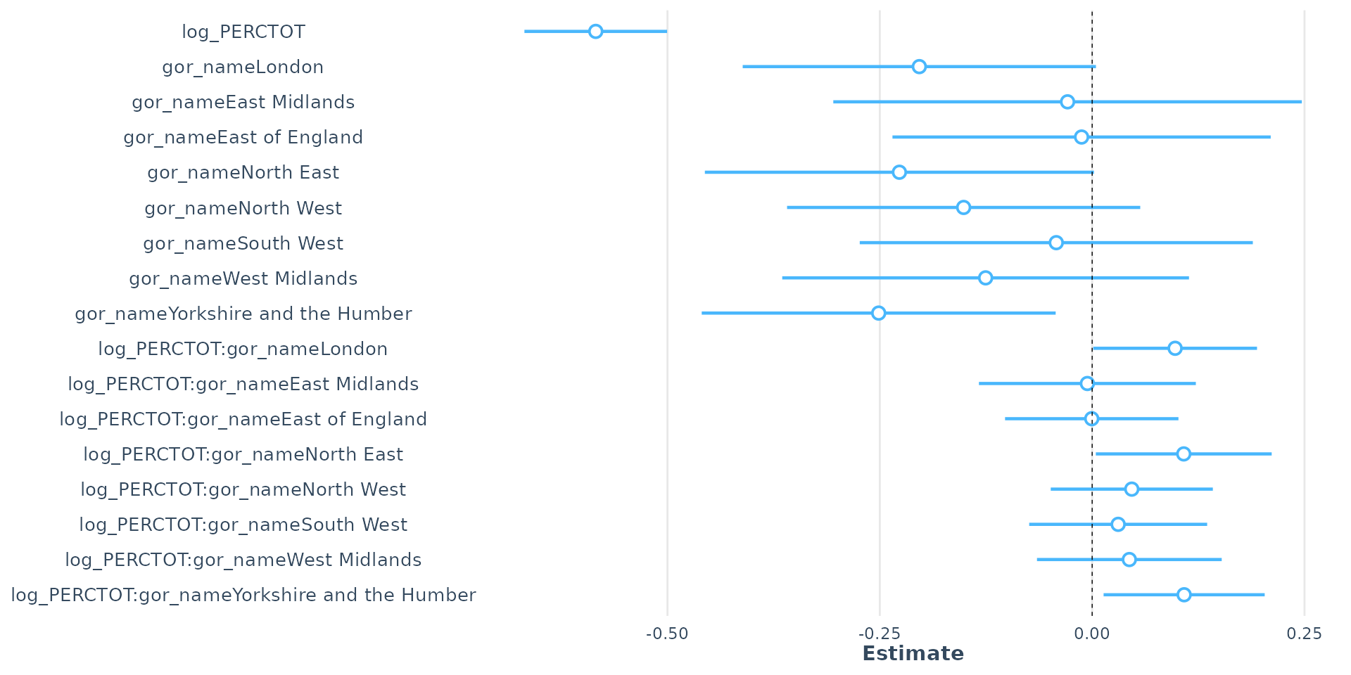
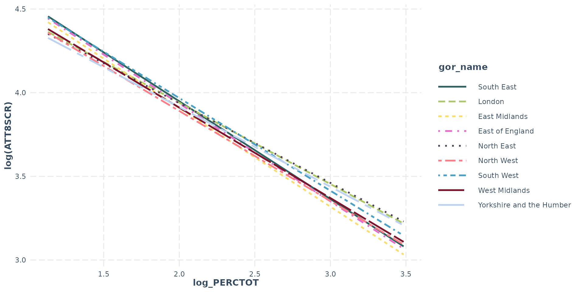
- 1% increase in the overall absence rate (log(PERCTOT)) predicts a 0.58% decrease in Attainment 8
- Controlling for overall absence, all other regions worse attainment than SE (reference). SE uniquely sensitive to absence
- Interaction effect: in London, NE & Yorkshire strong positive coefficient = negative effect of overall absence on attainment is significantly less severe than in SE
Interaction Effects
Interaction Effects
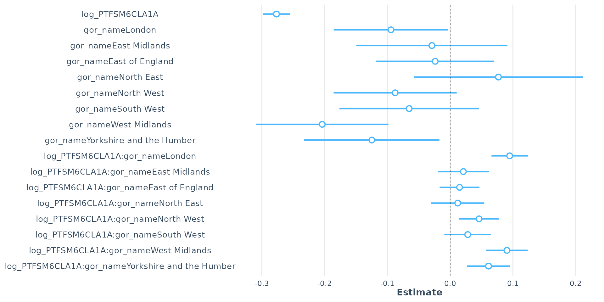
- Interacting disadvantage with region shows negative effect of disadvantage not as bad in regions other than SE - however…
Interaction Effects
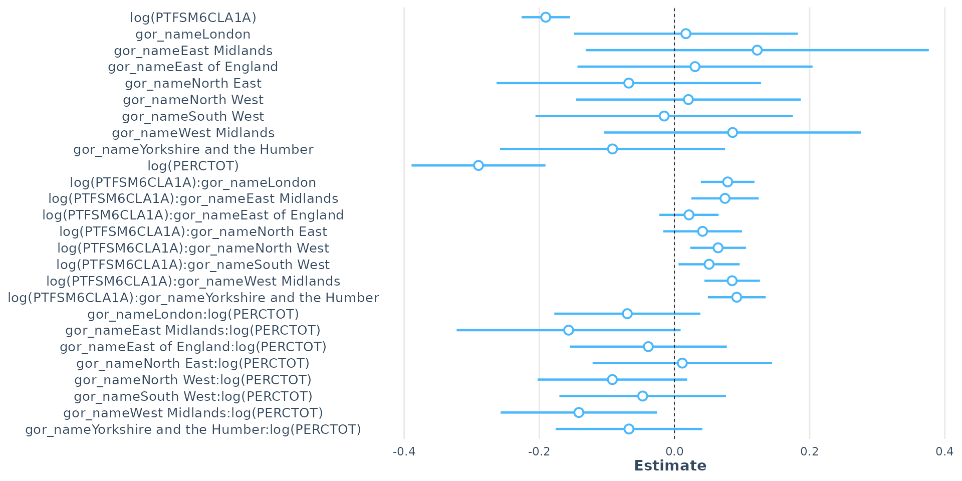
- As overall absence confounds disadvantage, so interacting both with region changes these effects
Interaction Effects
- Main Effect (Reference Group):
- The coefficient for log(PTFSM6CLA1A) is -0.190520. This is the effect of disadvantage in the South East.
- The coefficient for log(PERCTOT) is -0.289960. This is the effect of Overall Absence in the South East.
- Even when controlling for regional differences, unauthorised absence has a stronger negative effect on Attainment 8 than disadvantage
Interaction Effects
- Interaction Effects (Reference Group value + Other Region coefficient):
- log(PTFSM6CLA1A):gor_nameLondon: significant positive coefficient (+0.078684) - negative effect of disadvantage is less severe in London than in the South East
- same for all other regions - disadvantage has a more severe impact in the SE than anywhere else in England. SE schools particularly bad at mitigating effects of disadvantage
Interaction Effects
- Interaction Effects (Reference Group value + Other Region coefficient):
- gor_nameLondon:log(PERCTOT): The significant negative coefficient (-0.069792) - negative effect of Overall Absence is more severe in London than in the South East
- same for most other regions - Overall Absence as less severe impact in SE than anywhere else in England.
Interaction Effects
Call:
lm(formula = log(ATT8SCR) ~ log(PTFSM6CLA1A) * log(PERCTOT) +
    gor_name, data = model_data)

Residuals:
     Min       1Q   Median       3Q      Max
-1.24743 -0.05845  0.00082  0.06076  0.72702

Coefficients:
                                  Estimate Std. Error t value Pr(>|t|)
(Intercept)                       4.989742   0.064333  77.561  < 2e-16 ***
log(PTFSM6CLA1A)                 -0.125059   0.019674  -6.357 2.35e-10 ***
log(PERCTOT)                     -0.353934   0.032374 -10.933  < 2e-16 ***
gor_nameLondon                    0.095751   0.007137  13.417  < 2e-16 ***
gor_nameEast Midlands            -0.004420   0.007725  -0.572 0.567250
gor_nameEast of England           0.002028   0.007123   0.285 0.775845
gor_nameNorth East                0.075416   0.009864   7.646 2.72e-14 ***
gor_nameNorth West                0.004092   0.006853   0.597 0.550493
gor_nameSouth West                0.027349   0.007434   3.679 0.000238 ***
gor_nameWest Midlands             0.028953   0.007184   4.030 5.70e-05 ***
gor_nameYorkshire and the Humber  0.036074   0.007542   4.783 1.80e-06 ***
log(PTFSM6CLA1A):log(PERCTOT)    -0.003798   0.009586  -0.396 0.691945
---
Signif. codes:  0 '***' 0.001 '**' 0.01 '*' 0.05 '.' 0.1 ' ' 1

Residual standard error: 0.1025 on 3221 degrees of freedom
Multiple R-squared:  0.7182,    Adjusted R-squared:  0.7172
F-statistic: 746.2 on 11 and 3221 DF, p-value: < 2.2e-16- It is also possible to interact our continuous variables. However…
Interaction Effects
- Interaction term is statistically insignificant
- There is no evidence that the effect of concentrations of disadvantage on attainment changes based on the levels of unauthorised absence, or vice-versa
- Negative impact of disadvantage is roughly the same whether a school has a low or high unauthorised absence rate, and the negative impact of unauthorised absence is roughly the same regardless of the level of disadvantage
- Good to experiment as informative, but this interaction term can be removed from the model
Interaction Effects
- Final Note: Adding interaction effects will seriously increase your VIF as you are multiplying variables that are already in the model
- High VIF in a model with interaction terms does not affect the overall model.
- High VIF could inflate the standard errors of the coefficients making some otherwise significant variables seem insignificant
- Mean-Centring is a technique that could fix this, but we won’t look at it today
Interaction Effects
Tip
- Interpreting interaction effects is HARD (as you can probably tell from me trying to explain these!)
- AI is incredibly adept at interpreting outputs from regression models and describing the outputs in plain English. ChatGPT, Google Gemini, Claude and various others can be of great help here
- It doesn’t always get it right - never just feed an AI your outputs and trust its interpretation without questioning what it’s telling you
- Used correctly, however - particularly if you give it context with the data you are using and the patterns you are observing, it’s a tool that can really assist your understanding.
Some final thoughts on building regression models
- Aim is to try and explain as much variation in dependent variable as possible with the fewest number of independent variables
- More variables isn’t necessarily better - statistically insignificant variables might be worth dropping from your model
- As you add more variables, confounding might change the interpretation of earlier variables and may even stop them being statistically significant
- Algorithms like the Step-Wise algorithm can automate the process of variable selection - worth experimenting with, but no substitute for doing your own research!
- Building a good model takes time, experimentation, iteration and a lot of care and attention
Bringing it all together - our final regression show-stopper!
- In carefully building our regression model step-by-step, we have evolved our understanding:
- from a basic model for Brighton where it appeared that the % disadvantaged students in a school explained around 65% of the variation in Attainment 8 scores and a 10% decrease in disadvantage equating to a 6-point increase in Attainment 8
- to understanding that this initial local model was poor:
- few degrees of freedom
- unobserved confounding and mediation

Bringing it all together - our final regression show-stopper!
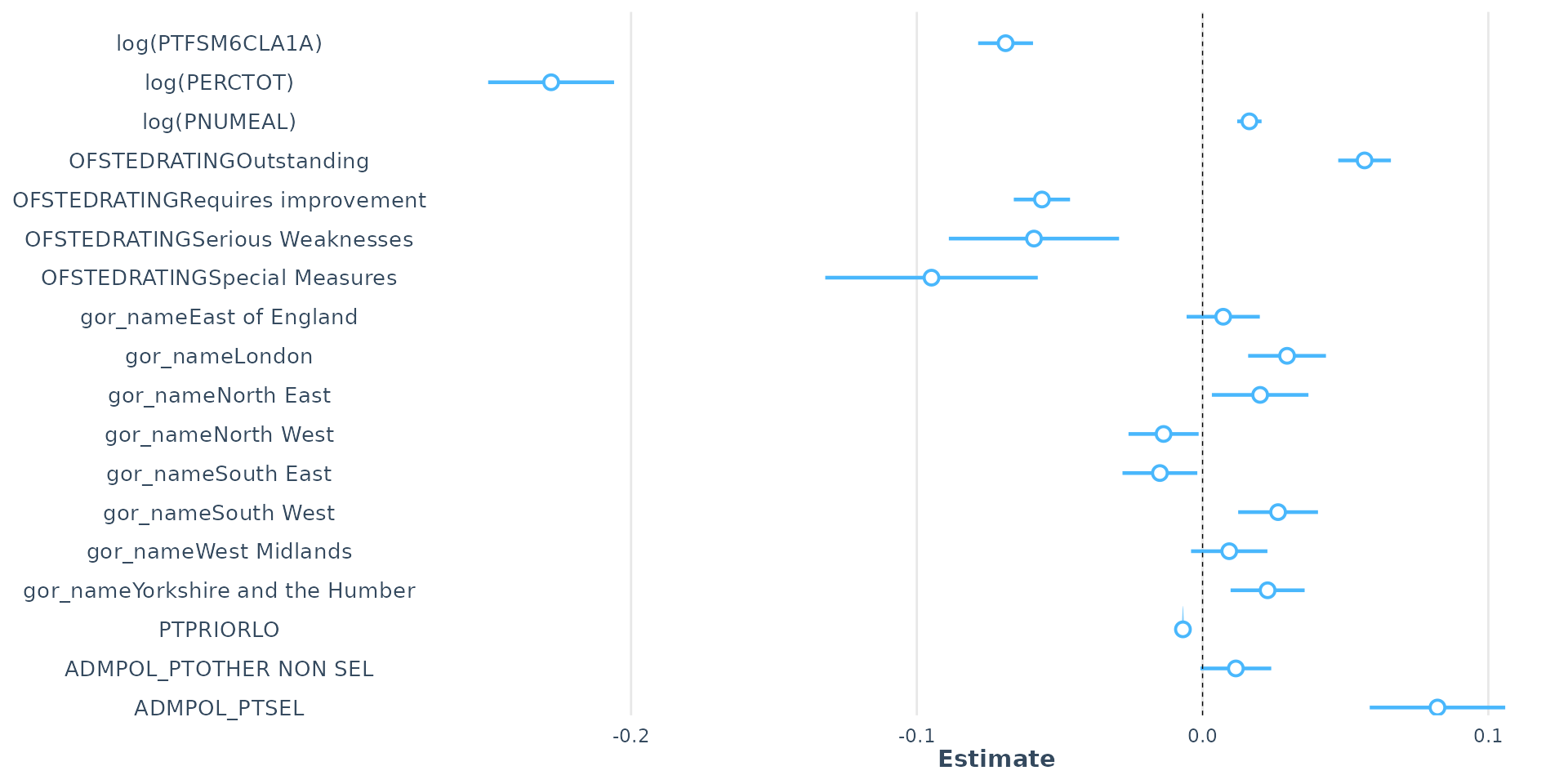
| R2 | R2 (adj.) | RMSE | Sigma |
|---|---|---|---|
| 0.83 | 0.83 | 0.08 | 0.08 |
Bringing it all together - our final regression show-stopper!
- Additional variables (some discussed, so not discussed in this lecture) have allowed us to explain almost 85% of the variation in Attainment 8 at the school level across England
- Careful interrogation of the coefficients as we have successively built up the complexity of the model reveals how the variables interact with each other
- The influence of disadvantage is partially confounded by overall absence
- but overall absence is a mediating variable in the relationship between disadvantage and attainment
Bringing it all together - our final regression show-stopper!
- Dummy variables can be your friend and allow us to compare how different groups perform in the data
- Ineracting variables can add even more explanatory power, but will take effort to interpret - AI can be your friend here if you are struggling
- If you follow the recipe, check you regression diagnostics at each stage and continually VISUALISE your data as you go, a good multiple regression model can be one of the most powerful explanatory tools in your toolbox!
This week’s practical
- Recreating much of what you have seen in this lecture yourself!
- Extending last week’s model and interpreting the outputs in Python or R
- This is another long practical - you won’t complete it in class today, so you should spend time at home (while listening to the Progression Sessions, preferably) working through this at your own pace.
- It is important that you are able to build your best model before next week’s lecture and practical session!

© CASA | ucl.ac.uk/bartlett/casa