Linear Algebra

Bea Taylor - beatrice.taylor@ucl.ac.uk

27th October 2026

Last week

Lecture 3 - hypothesis testing

Looked at:

• What makes a good hypothesis
• How to formally state a hypothesis
• Types of statistical tests

This week

Back to the starting point - Maths!

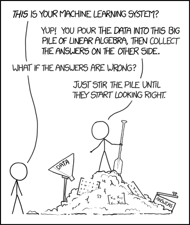
Image credit: [xkcd](https://xkcd.com/1838/)

• quantitative methods include data analysis and machine learning
• mostly focused on methodologies
• AND practical examples of how these can be applied
• BUT helpful to understand the underlying mathematics

This week focussing on the maths. Not going to be directly examined on the maths - this isn’t a maths course.

Rather the idea is to help with the basics which will facilitate understanding of subsequent weeks.

Maths doesn’t bite!

Maths can seem scary – but goal is to have a better understanding of key ideas. Going to cover quite abit - so focus on the goal of being able to understand equations.

Not expecting students to be experts!

Learning Objectives

By the end of this lecture you should be able to:

1. Define concept of linear equations.
2. Compute linear algebra equations using vectors and matrices.
3. Translate mathematical equations into plain English.
   

Motivation

What does it mean?

The goal is to understand equations like this:

\[\begin{align} y = \sum_{i=1}^n \beta_i x_i \end{align}\]

This is a standard linear equation.

But what does it mean???

Equations are often used in the methods sections of papers to describe the model.

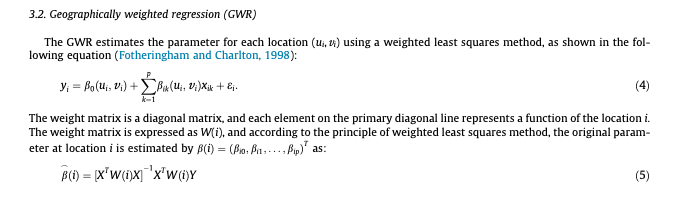
Taken from: Chiou, Jou, & Yang, (2015). Factors affecting public transportation usage rate: Geographically weighted regression. Transportation Research Part A: Policy and Practice.

This is an equation for a geographically weighted regression model.

Basics

Mathematical models

• Mathematical models help us to understand the data
• In a regression setting the model describes a function that maps input to real-valued outputs
• We can use mathematical models to validate our hypotheses/research questions

Thinking back to hypotheses from last week - mathematical models help us to evaluate our research question. Lats week we looked at simple statistical tests - but might have a more sophisticated model of what’s happening.

Example is a regression model (which we’ll look at after reading week) - this is a mathematical model

Machine learning

A model which improves after data is taken into account.

• Many of these concepts are also integral to machine learning
• Really just a specific type of mathematical model
• The learning part is about automatically finding patterns

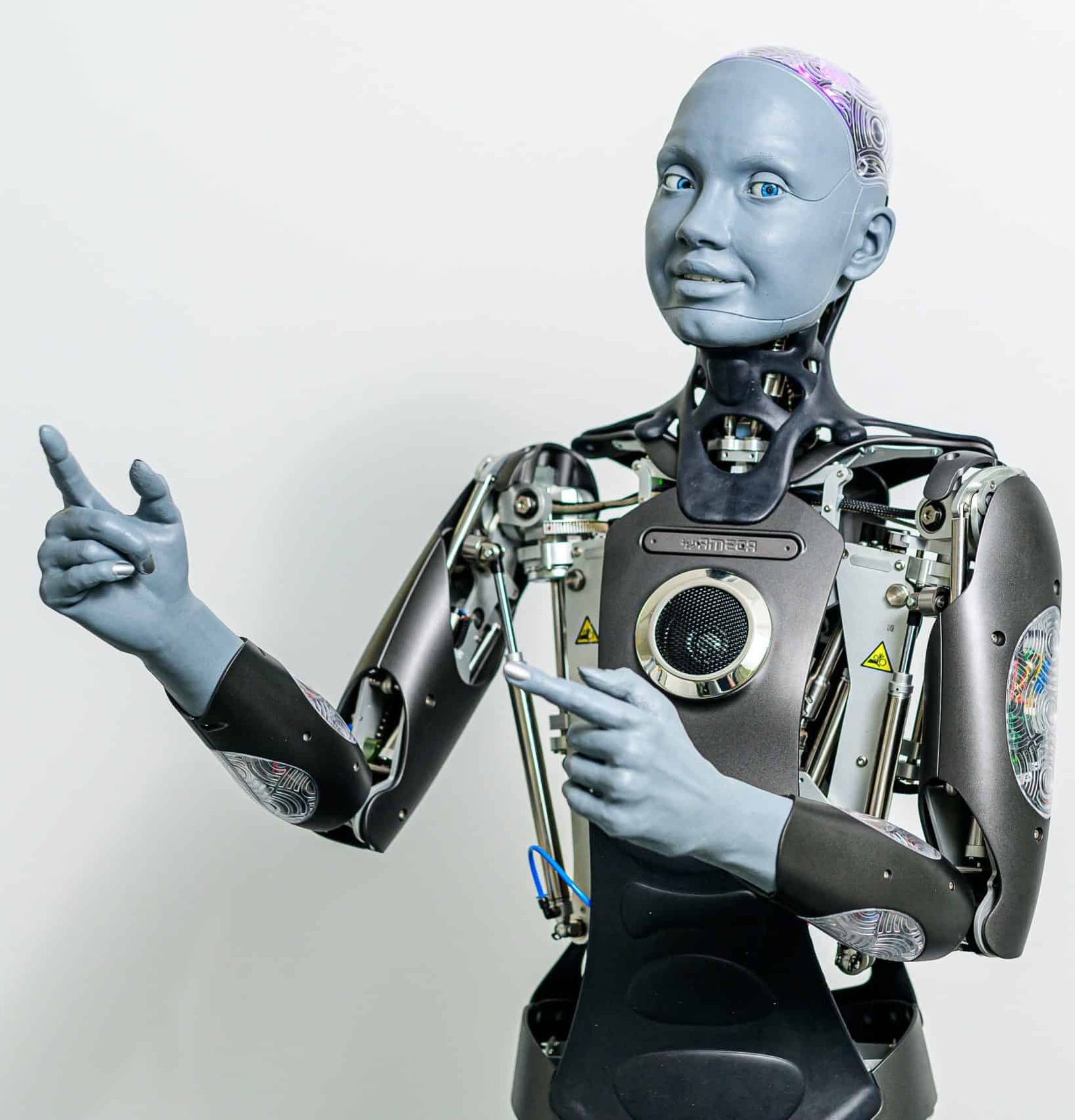
Embodied AI in the form of the creepy Ameca. 

These ideas are also fundamental for machine learning.

Lots of different definitions of machine learning - but this us a simple one - machine learning is a sub discipline of AI.

In later weeks of the course we will look at machine learning concepts, such as clustering.

Notation

Mathematical notation

Going to be using some mathematical notation

• as this is what’s used in papers!

It’s just a formal way of writing maths.

Provides a universal way of writing and understanding maths.

Cheat sheet

Mathematical notation cheat sheet

Letters for numbers

There are mathematical conventions for how we describe different things.

• \(a, b, c\) represent constants/coefficients
  
• \(x, y, z, \dots\) represent variables
  
• \(f, g, h, \dots\) represent functions
  
• \(i, j, \dots\) often used for indices (i.e. counting)
  • \(a_i\) means the \(i\)-th element of a sequence
    
• \(A, B, C, \dots\) represent matrices

Write up on board f(x)=ax_1 + bx_2 + c Explain the menaing of this equation.

Numbers replaced by letters

The power to represent any number!

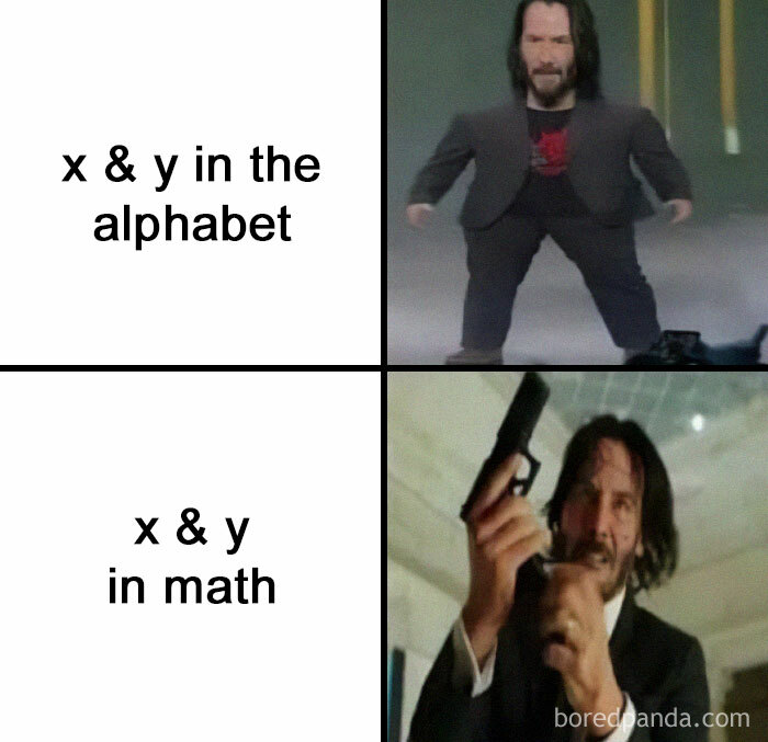
Keanu likes algebra. 

This is powerful as it allows is to represent abstract concepts - a universal x, rather than a specific number.

Sums

Summation notation is a compact way to write repeated addition.

\[\begin{align} \sum_{i=1}^n a_i = a_1 + a_2 + a_3 + \dots + a_n \end{align}\]

Example:

\[\begin{align} \sum_{i=1}^5 i = 1+2+3+4+5 = 15 \end{align}\]

Product

Product notation is a compact way to write repeated multiplication.

\[\begin{align} \prod_{i=1}^n a_i = a_1 \cdot a_2 \cdot a_3 \cdot \dots \cdot a_n \end{align}\]

Example:

\[\begin{align} \prod_{i=1}^4 i = 1 \cdot 2 \cdot 3 \cdot 4 = 24 \end{align}\]

a little bit of epsilon

\(\epsilon\) is used to mean a small, but arbitrary, number.

Example:

\[\begin{align} y = 2x + \epsilon \end{align}\]

This means \(y\) is equal to \(2\) times \(x\) plus a small value. So if \(x=3\), then we would expect \(y\) to be close to \(6\), but not exactly \(6\).

Could talk about it here in terms of the limit of a sequence, 1, 1.5, 1.25, 1.125, 1.0125, … the limit is 1, but it never reaches 1, the values will always be 1 + epsilon.

Functions

What is a function?

A function is a mathematical operation which maps an input value to an output value.

Mathematical description of a function

\[\begin{align} f(x) = y \end{align}\]

Maps values from a domain \(X\) to a range \(Y\).

\[\begin{align} f(x) = y \text{ for } x \in X, y \in Y \end{align}\]

explain the ‘in’ notation if not already.

Domain and range

Domain - the set of all possible input numbers for the function

Example:

In \(f(x)=y\), \(x\) is the domain.

Range: the set of all possible output numbers from the function

Example:

In \(f(x)=y\), \(y\) is the range.

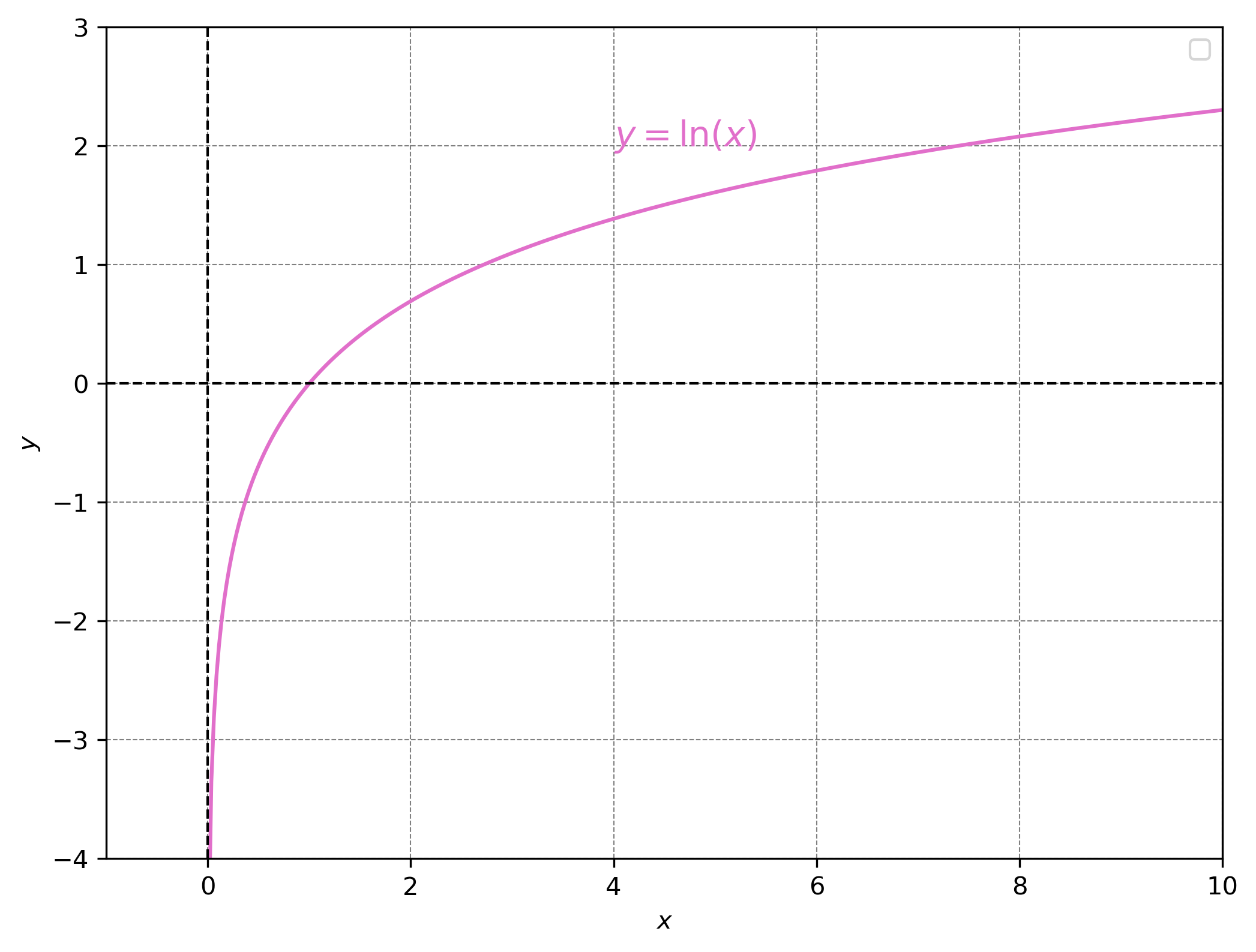
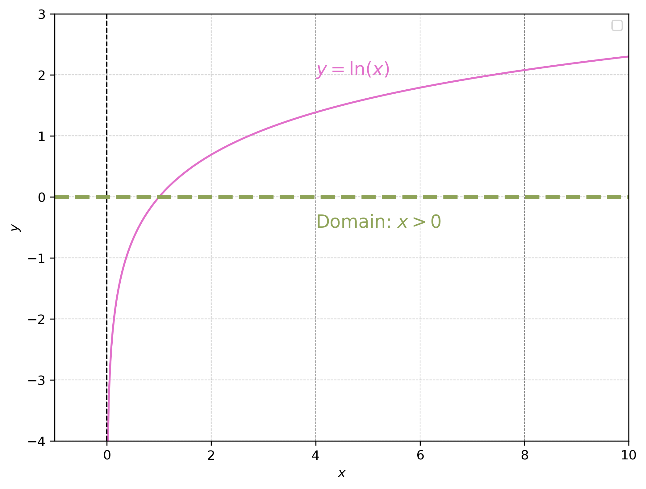
Question: what is the domain of \(ln(x)\)?

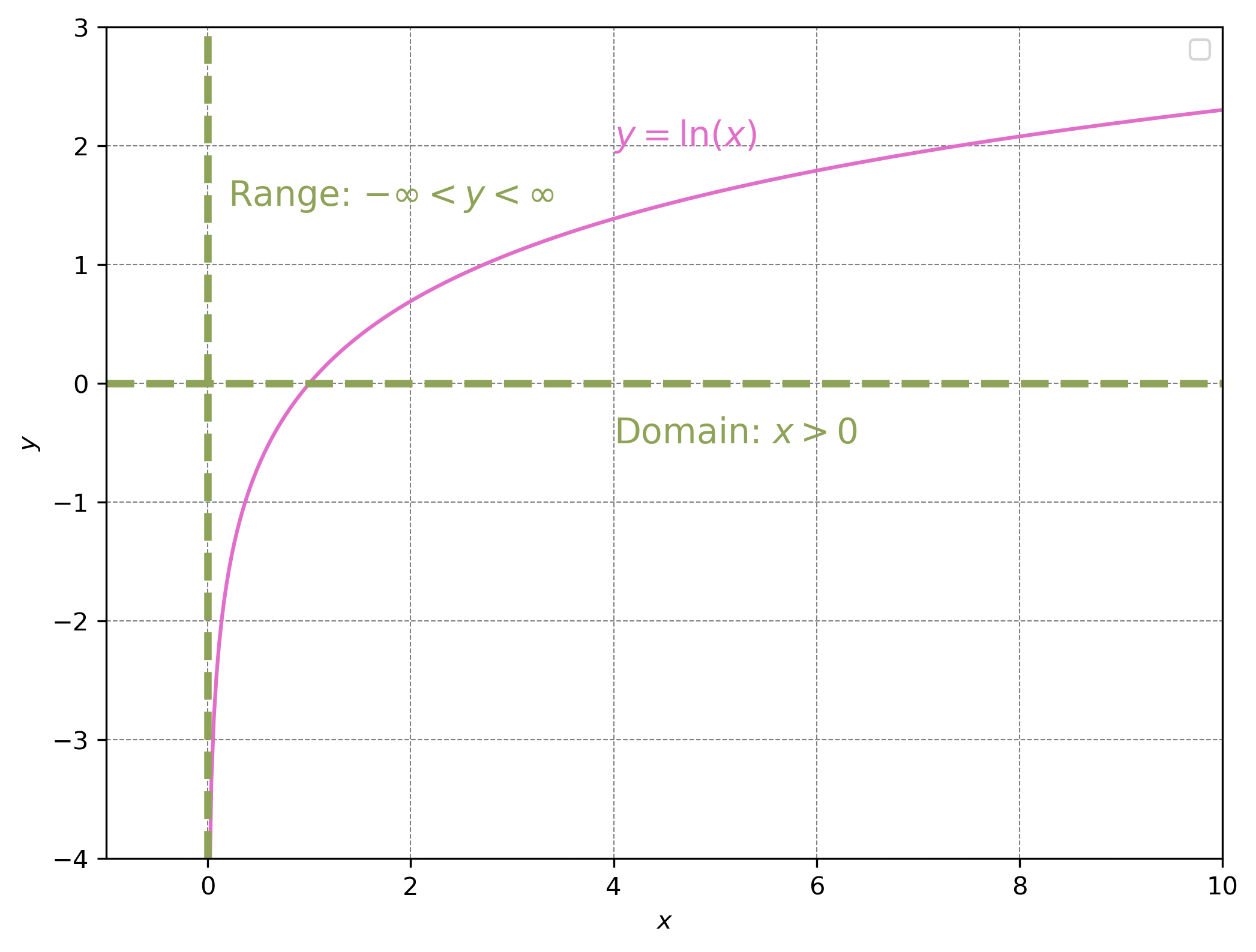
Question: what is the range of \(ln(x)\)?

Number systems

In the applied sciences the domain and range are typically \(\mathbb N\) or \(\mathbb Z\) or \(\mathbb R\)

• \(\mathbb N\) - Natural numbers
  • 0,1,2,3,4,5,6…
• \(\mathbb Z\) - Integers
  • … -4, -3, -2, -1, 0, 1, 2, 3, 4, …
• \(\mathbb R\) - Real numbers

The natural number are the counting numbers. The integers are the natural number extended into negative values. Then have rational numbers - which is anything that can be represented by a fraction. Finally the real numbers - think of as all numbers - so includes those which can’t be repesented by fractions, e.g. pi.

Data represented algebraically

Algebra is a way of expressing numbers in a generalised or abstract form.

Example:

\[\begin{align} x \in \mathbb N \end{align}\]

• This is the data represented algebraically.
• A vector of numbers \(X^n\)

\[\begin{align} X^n = (x_1, x_2, x_3, ... , x_n) \end{align}\]

Example 1

Probability density function of normal distribution

\[\begin{align} f(x) = \frac{1}{\sqrt{2 \pi \sigma^2}} e^{-\frac{(x-\mu)^2}{2\sigma^2}} \end{align}\]

where \(x \in \mathbb R\) and \(f(x) \in [ 0 , 1 ]\).

Note

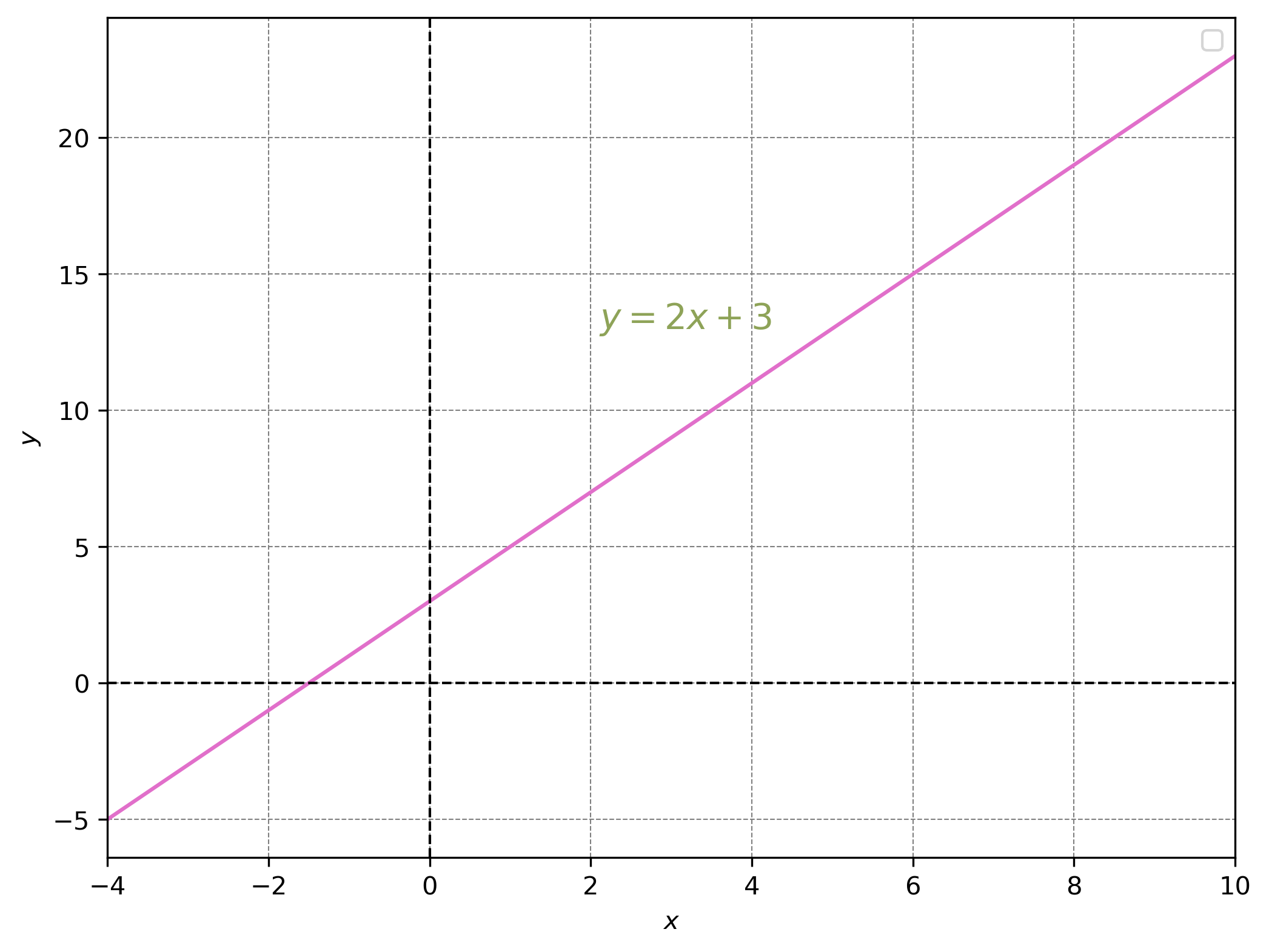
\([0, 1]\) is the set of real numbers between \(0\) and \(1\), inclusive of \(0\) and \(1\).

In week 2 we were thinking about PDFs - these are a function. They map the input value, the ‘x’ to the output range which is a probability between 0 and 1.

Example 2

The other function we’ve seen is a linear equation.

\[\begin{align} f(x) = ax + b \end{align}\]

Going to spend the rest of the lecture looking at linear algebra - i.e. algebra related to linear equations.

Break

Linear equations

Linear equation

A linear equation is a linear combination of variables.

Examples include:

\[\begin{align} f(x) = ax + b \end{align}\]

“linea” is the latin word for line or string.

Straight lines

Graphically linear equations are straight lines.

Linear equation(s)

We can generalise to multiple equations.

They are:

• A system of multiple linear functions
• Which can be represented by matrices
• They can have 0, 1, or many solutions

Example 1

\[\begin{align} x+y=10 \end{align}\]

• What could \(x\) and \(y\) be?
• Could have \(x=y=5\)
• Or \(x=2.5\) and \(y=7.5\)

There are many solutions!!!

Many solutions = under-specified

Under-specified means there isn’t enough information to find a unique solution.

Under-specified but simple to solve!

Under-specified means I don’t have enough information to find a unique solution.

Example 2

\[\begin{align} x+y=10 \\ 2x+y=15 \end{align}\]

In school might have solved this using substitution.

• Rearrange the first equation to get \(y=10-x\)
• Substituting in we get \(2x+(10-x)=15\)
• \(x+10=15\) \(\implies\) \(x=5\) \(\implies\) \(y=5\)

There is exactly one solution!

Perfectly specified and we can solve it without too much difficulty

Example 3

\[\begin{align} x_1+x_2+x_3+x_4=10 \\ x_1+4x_2+x_3+x_4=25 \\ x_1+4x_2+43x_3+x_4=37 \\ x_1+4x_2+7x_3+59x_4=1073 \end{align}\]

Very hard to solve!

An example (when things get more complicated)

Matrices

Matrix notation

\[\begin{align} x_1+x_2+x_3+x_4=10 \\ x_1+4x_2+x_3+x_4=25 \\ x_1+4x_2+43x_3+x_4=37 \\ x_1+4x_2+7x_3+59x_4=1073 \end{align}\]

Can be written as:

\[\begin{align} \begin{bmatrix}1&1&1&1\cr1&4&1&1\cr1&4&43&1\cr1&4&7&59\end{bmatrix}\begin{pmatrix}x_1\cr x_2\cr x_3\cr x_4\end{pmatrix} = \begin{pmatrix}10\cr 25\cr 37\cr 1073\end{pmatrix} \end{align}\]

Generalised matrix form

The generalised matrix form (for a 4x4 matrix is):

\[\begin{align} \begin{bmatrix}a_{1,1} & a_{1,2} & a_{1,3} & a_{1,4}\cr a_{2,1} & a_{2,2} & a_{2,3} & a_{2,4}\cr a_{3,1} & a_{3,2} & a_{3,3} & a_{3,4}\cr a_{4,1} & a_{4,2} & a_{4,3} & a_{4,4}\end{bmatrix}\begin{pmatrix}x_1\cr x_2\cr x_3\cr x_4\end{pmatrix} = \begin{pmatrix}y_1 \cr y_2 \cr y_3 \cr y_4\end{pmatrix} \end{align}\]

Down the stairs, along the corridor

Matrices are indexed by row (\(m\)) and by column (\(n\)).

Example

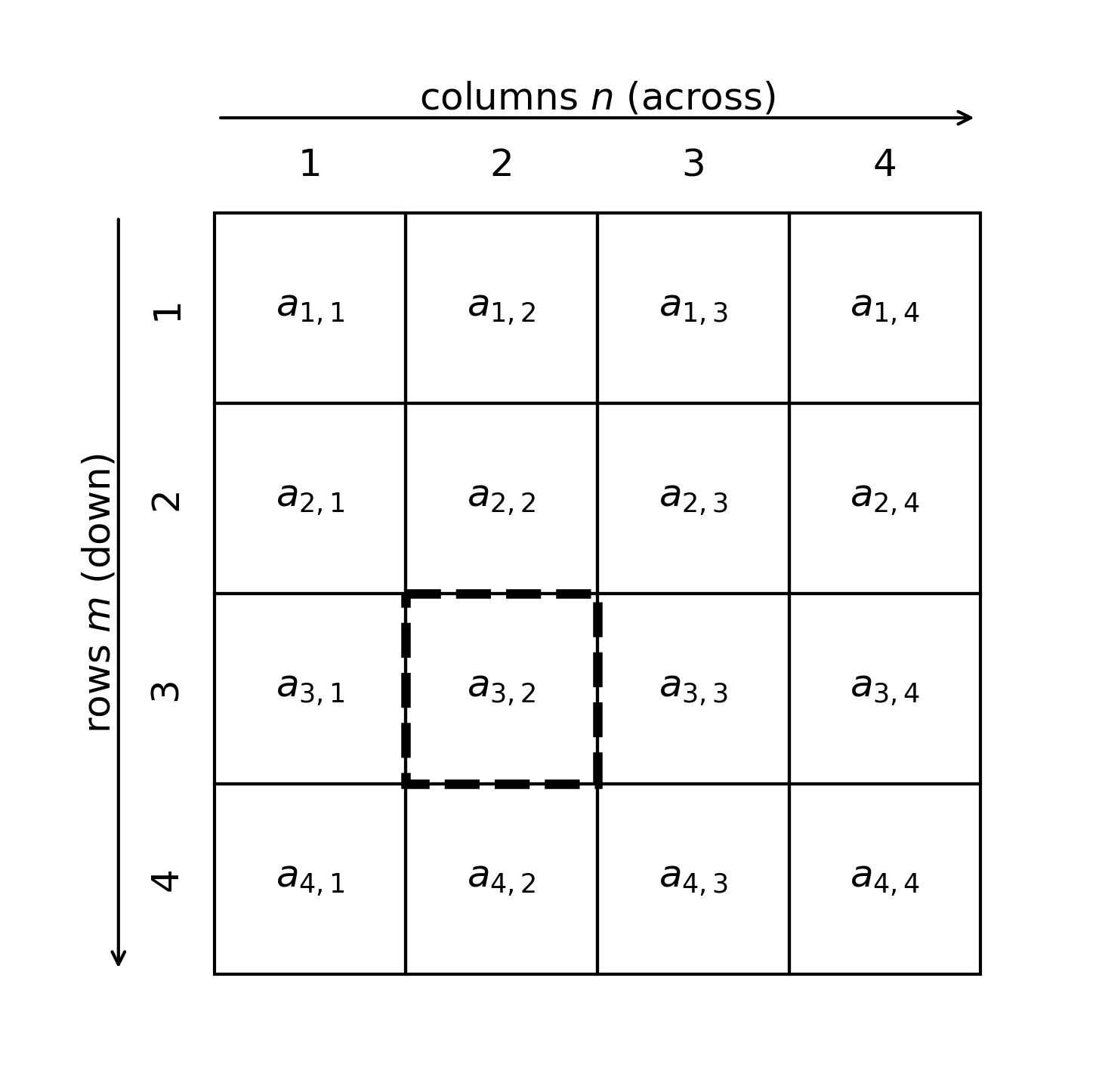
\(m=2\), \(n=2\) matrix:

\[\begin{align} \begin{bmatrix}1&1\cr1&4\end{bmatrix} \end{align}\]

\(m=2\), \(n=3\) matrix:

\[\begin{align} \begin{bmatrix}1&1&2\cr1&4&7\end{bmatrix} \end{align}\]

Note

When \(m=n\) we have a square matrix.

Matrix addition

We denote matrices by capital letters: \(A\), \(B\), …

Matrix addition is element-wise:

\[\begin{align} (A+B)_{ij} = A_{ij} + B_{ij} \end{align}\]

Example:

\[\begin{align} \begin{bmatrix}1&1\cr1&4\end{bmatrix} + \begin{bmatrix}1&0\cr2&6\end{bmatrix} = \begin{bmatrix}2&1\cr3&10\end{bmatrix} \end{align}\]

Matrix multiplication

Matrix multiplication is row by column.

\[\begin{align} (AB)_{ij} = \sum_{k} A_{ik} B_{kj} \end{align}\]

Where \(k\) is the dimension of the matrix.

Example:

\[\begin{align} \begin{bmatrix}1 & 2\cr 3 & 4\end{bmatrix} \begin{bmatrix}5 & 6\cr 7 & 8\end{bmatrix} = \begin{bmatrix} 1\cdot 5 + 2\cdot 7 & 1\cdot 6 + 2\cdot 8 \cr 3\cdot 5 + 4\cdot 7 & 3\cdot 6 + 4\cdot 8 \end{bmatrix} = \begin{bmatrix} 19 & 22 \cr 43 & 50 \end{bmatrix} \end{align}\]

Matrix multiplication rule

The dimensions of the matrices need to match in order to multiple them.

Generally I can multiply \(A\) by \(B\) if \(A\) has the same number of columns as \(B\) has rows.

If:

\[\begin{align} dim(A)=m \times n \\ dim(B)=n \times l \end{align}\]

Then:

\[\begin{align} dim(AB)=m \times l \end{align}\]

Write this out on the board - collapsing the middle dimensions

Transpose of a matrix

When you take the transpose of matrix you flip it through it’s diagonal.

For

\[\begin{align} A = \begin{bmatrix} a & b \cr c & d \end{bmatrix} \end{align}\]

then,

\[\begin{align} A^T = \begin{bmatrix} a & c \cr b & d \end{bmatrix} \end{align}\]

Could do example for a non-square matrix on the board.

Identity matrix

The identity matrix \(I\) acts like the number \(1\) in multiplication.

For any compatible matrix \(A\):

\[\begin{align} AI = IA = A \end{align}\]

Example:

\[\begin{align} I = \begin{bmatrix} 1 & 0 & 0 \cr 0 & 1 & 0 \cr 0 & 0 & 1 \end{bmatrix} \end{align}\]

Determinant of a matrix

The determinant of a square matrix \(A\) is a scalar value that gives information about:

• Whether \(A\) is invertible
  
• How \(A\) scales space (volume/area)
  
• Orientation (positive or negative)

We write this as \(\det(A)\) or \(|A|\).

Determinant of a 2×2 matrix

For

\[\begin{align} A = \begin{bmatrix} a & b \cr c & d \end{bmatrix} \end{align}\]

the determinant is:

\[\begin{align} \det(A) = ad - bc \end{align}\]

Example:

\[\begin{align} det( \begin{bmatrix} 1 & 2 \cr 3 & 4 \end{bmatrix} ) = 1 \times 4 - 2 \times 3 = -2 \end{align}\]

Inverse matrix

The inverse of a square matrix \(A\) is denoted \(A^{-1}\) and satisfies:

\[\begin{align} AA^{-1} = A^{-1}A = I \end{align}\]

Inverse matrix (2x2)

For a \(2 \times 2\) matrix A:

\[\begin{align} A = \begin{bmatrix} a & b \cr c & d \end{bmatrix} \end{align}\]

if \(\det(A) \neq 0\), then the inverse is:

\[\begin{align} A^{-1} = \frac{1}{\det(A)} \begin{bmatrix} d & -b \cr -c & a \end{bmatrix}, \quad \text{where } \det(A) = ad - bc \end{align}\]

If \(\det(A) = 0\), the matrix has no inverse.

System of equations

Recall that a system of linear equations can be written compactly as:

\[\begin{align} Ax = y \end{align}\]

where:

• \(A\) is the coefficient matrix
• \(x, y\) are variables in vector form

Solving the system

If \(A\) is invertible (i.e. \(\det(A) \neq 0\)), we can solve for \(x\):

\[\begin{align} Ax &= y \\ A^{-1}Ax &= A^{-1}y \\ Ix &= A^{-1}y \\ x &= A^{-1}y \end{align}\]

Thus, the solution exists and is unique whenever \(A\) has an inverse.

The exciting bit - we can bring all the ideas we’ve seen together in order to solve the equation.

Maths to English

Using what we’ve learnt to interpret equations

How can we translate it? Going to look at an equation and use what we’ve done to try and understand it.

So what does it mean?

Taken from: Chiou, Jou, & Yang, (2015). Factors affecting public transportation usage rate: Geographically weighted regression. Transportation Research Part A: Policy and Practice.

I’ve chosen quite an arbitrary paper - which includes an equation for geographically weigthed regression. Using and solving regression is going to be covered after reading week.

But today we’re going to look at ‘reading the maths’.

Take another look

Chiou, Jou, & Yang, (2015). Factors affecting public transportation usage rate: Geographically weighted regression. Transportation Research Part A: Policy and Practice.

Writing the equation

Equation 1:

\[\begin{align} y_i = \beta_0(u_i, v_i) + \sum_{k=1}^p \beta_{ik}(u_i, v_i)x_{ik} + \epsilon_i \end{align}\]

Equation 2:

\[\begin{align} \hat{\beta}(i) = [X^TW(i)X]^{-1}X^TW(i)Y \end{align}\]

Question: What do you think these equations mean?

Write out a simplified version on the board - and ask students what they think the equations might mean.

Equation 1: linear equation

Equation 2: tells us how to estimate beta - its a product of matrices

Equation 1

\[\begin{align} y_i = \beta_0(u_i, v_i) + \sum_{k=1}^p \beta_{ik}(u_i, v_i)x_{ik} + \epsilon_i \end{align}\]

where:

• \(y_i\) is the outcome (response) for observation \(i\)
• \(u_i,v_i\) is the location
• \(\beta_0(u_i,v_i)\) is the intercept, which can vary with location \((u_i,v_i)\)
• \(\beta_{ik}(u_i,v_i)\) are coefficients depending on \((u_i,v_i)\)
• \(\sum_{k=1}^p \beta_{ik}(u_i,v_i) x_{ik}\) is the weighted sum of predictor variables \(x_{ik}\), where each predictor has its own coefficient that may depend on \((u_i,v_i)\)
• \(\epsilon_i\) the error term for observation \(i\)

Read the equation out - and then break down each part of the equation

Translating equation 1

\[\begin{align} y_i = \beta_0(u_i, v_i) + \sum_{k=1}^p \beta_{ik}(u_i, v_i)x_{ik} + \epsilon_i \end{align}\]

In plain english:

The outcome \(y_i\) is explained by an intercept and a weighted combination of predictors, with coefficients that may change depending on the location \((u_i,v_i)\), plus some error.

This is exactly a linear equation - but the coefficients are allowed to vary with location.

We solve linear equatiosn usign linear regression - which is what we’ll see next week.

Equation 2

\[\begin{align} \hat{\beta}(i) = [X^TW(i)X]^{-1}X^TW(i)Y \end{align}\]

where:

• \(X\): the matrix of predictor variables
• \(Y\): the vector of observed outcomes
• \(W(i)\): a weight matrix that depends on location \(i\) - it is weighted so that observations nearer to \(i\) have greated weight
• \(X^T\): the transpose of \(X\)
• \([X^TW(i)X]^{-1}\): the inverse of the weighted cross-product matrix

Read the equation out

Translating equation 2

\[\begin{align} \hat{\beta}(i) = [X^TW(i)X]^{-1}X^TW(i)Y \end{align}\]

In plain english:

We estimate the coefficients \(\hat{\beta}(i)\) by solving a weighted least squares problem: take the predictors \(X\), weight them with \(W(i)\), and solve for the coefficients that best fit \(Y\).

Overview

Covered

We’ve covered:

• Mathematical notation
• Sums and Products
• Functions
• Matrices
• Algebraic representations

Key takeaways

• Can use mathematical notation to write equations in a univeral language.
• Linear algebra helps us to solve systems of linear equations.

If in doubt:

Use the maths cheat sheet!

Practical

The practical will focus on understanding mathematical equations.

• Have questions prepared!