Prof D’s Regression Sessions - Vol 4

Good Skool / Bad Skool Breaks - a logistic regression walkthrough

Author

Adam Dennett

Published

Invalid Date

Preamble

Three volumes of the Regression Sessions have all relied on the idea that the thing we are trying to predict is a continuous number. That number can wander up and down a straight line without ever embarrassing us by predicting something mad!

It’s one of the core assumptions of ordinary least squares linear regression, but today we are going to break it. Our outcome is a yes/no: is this school rated below Good by Ofsted? A straight line is the wrong tool for that job, and the first task of the practical is to watch it fail - properly, on real data, with numbers you can point at - before we reach for a totally different tool that fixes it.

Practical aims

Fit a linear probability model to a 0/1 outcome and find its impossible predictions
Fit, and read, a binary logistic regression - including saying an odds ratio out loud in a sentence a non-statistician would understand
Judge the fit with deviance, AIC and the pseudo-R²s
Judge the decisions honestly: against a baseline, with a confusion matrix, and with ROC and AUC
Take at least one of the two extensions further than the lecture went

Before you start: the two tabs

Every code block below has an R tab and a Python tab. They are not loose translations of each other - they do the same arithmetic on the same rows and produce the same numbers, to four decimal places, all the way through. If your two tabs disagree, something has gone wrong, and that is worth chasing down.

Keep the whole thing reproducible

We split the data into training and test sets using the row position after sorting by URN, not a random number generator. That is deliberate: R’s sample() and Python’s random number generators will never agree with one another, and you would spend the afternoon wondering why your AUC was not mine. Sorting and taking every tenth school is boring, reproducible, and gives the same 2,219 training and 951 test schools in both languages.

Part 0: The data

Task 0 - Load the schools data and build the outcome

We use the same four DfE files as the lecture. Three things are happening here that are worth noticing rather than skimming:

Rows with no URN are dropped. The files carry local authority and national summary rows that are not schools. They also duplicate rows on a join, because a missing key matches another missing key.
Ofsted’s five published grades collapse to a binary. below_good is 1 for Requires improvement, Serious Weaknesses and Special Measures, and 0 for Good and Outstanding.
We keep mainstream secondaries only, so that we are comparing schools that are doing roughly the same job.
Also note how we generate a new binary variable from OFSTEDRATING for schools that are below Good and the rest. This is created differently in R and Python.

Code

library(tidyverse)
library(here)

base_path <- here("sessions", "data", "Performancetables_130242", "2022-2023")

# The DfE publishes suppressed / not-applicable values as codes, not blanks
na_all <- c("", "NA", "SUPP", "NP", "NE", "SP", "SN", "LOWCOV", "NEW", "SUPPMAT")

read_dfe <- function(f) {
  suppressWarnings(
    read_csv(file.path(base_path, f), na = na_all, show_col_types = FALSE)
  ) |>
    mutate(URN = as.character(URN)) |>
    filter(!is.na(URN))
}

ks4 <- read_dfe("england_ks4final.csv") |>
  select(URN, ATT8SCR, P8MEA, TPUP, PTFSM6CLA1A, PTPRIORHI) |>
  mutate(across(-URN, ~ parse_number(as.character(.x))))

absence <- read_dfe("england_abs.csv") |>
  distinct(URN, .keep_all = TRUE) |>
  select(URN, PERCTOT, PPERSABS10) |>
  mutate(across(-URN, ~ parse_number(as.character(.x))))

school_info <- read_dfe("england_school_information.csv") |>
  select(URN, SCHNAME, LANAME, MINORGROUP, OFSTEDRATING)

schools <- ks4 |>
  inner_join(absence, by = "URN") |>
  inner_join(school_info, by = "URN") |>
  filter(MINORGROUP %in% c("Academy", "Maintained school"),
         OFSTEDRATING %in% c("Outstanding", "Good", "Requires improvement",
                             "Serious Weaknesses", "Special Measures")) |>
  mutate(below_good = as.integer(
    OFSTEDRATING %in% c("Requires improvement", "Serious Weaknesses",
                        "Special Measures")))

# Complete cases only, sorted, so the split below is reproducible
model_data <- schools |>
  drop_na(P8MEA, PTFSM6CLA1A, PERCTOT, PPERSABS10, TPUP, PTPRIORHI) |>
  arrange(URN)

nrow(model_data)

[1] 3170

Code

mean(model_data$below_good)

[1] 0.1498423

Code

import pandas as pd
import numpy as np
from pathlib import Path

# Little function to find the project root on any machine
def find_qm_root(start_path: Path = Path.cwd(), anchor: str = "_quarto.yml") -> Path:
    for parent in [start_path] + list(start_path.parents):
        if (parent / anchor).exists() or parent.name == anchor:
            return parent
    raise FileNotFoundError(f"Anchor '{anchor}' not found in path hierarchy.")

qm_root = find_qm_root()
base_path = qm_root / "sessions" / "data" / "Performancetables_130242" / "2022-2023"

na_all = ["", "NA", "SUPP", "NP", "NE", "SP", "SN", "LOWCOV", "NEW", "SUPPMAT"]

def read_dfe(f, cols):
    d = pd.read_csv(base_path / f, na_values=na_all, dtype={"URN": str},
                    low_memory=False)
    return d[d["URN"].notna()][cols]

def to_num(df, cols):
    for c in cols:
        df[c] = pd.to_numeric(df[c].astype(str).str.replace("%", "", regex=False),
                              errors="coerce")
    return df

ks4 = read_dfe("england_ks4final.csv",
               ["URN", "ATT8SCR", "P8MEA", "TPUP", "PTFSM6CLA1A", "PTPRIORHI"])
ks4 = to_num(ks4, ["ATT8SCR", "P8MEA", "TPUP", "PTFSM6CLA1A", "PTPRIORHI"])

absence = read_dfe("england_abs.csv", ["URN", "PERCTOT", "PPERSABS10"]) \
            .drop_duplicates("URN")
absence = to_num(absence, ["PERCTOT", "PPERSABS10"])

school_info = read_dfe("england_school_information.csv",
                       ["URN", "SCHNAME", "LANAME", "MINORGROUP", "OFSTEDRATING"])

schools = ks4.merge(absence, on="URN").merge(school_info, on="URN")
schools = schools[schools["MINORGROUP"].isin(["Academy", "Maintained school"])]
schools = schools[schools["OFSTEDRATING"].isin(
    ["Outstanding", "Good", "Requires improvement",
     "Serious Weaknesses", "Special Measures"])]
schools["below_good"] = schools["OFSTEDRATING"].isin(
    ["Requires improvement", "Serious Weaknesses", "Special Measures"]).astype(int)

model_data = (schools
    .dropna(subset=["P8MEA", "PTFSM6CLA1A", "PERCTOT", "PPERSABS10",
                    "TPUP", "PTPRIORHI"])
    .sort_values("URN")
    .reset_index(drop=True))

print(len(model_data))

Code

print(model_data["below_good"].mean())

0.1498422712933754

Check before you go on

You should have 3,170 schools, and 15.0% of them below Good. If you have a different number, your filters have not matched mine and every figure below will drift.

15% is the number to remember

Only 15 schools in 100 are below Good. Write that down. It is going to come back and ruin our afternoon at Task 10, in the most instructive way possible.

Part 1: Watching a straight line fail

Task 1 - Fit the linear probability model

Before we do anything clever, do the obvious wrong thing. below_good is a column of 0s and 1s, and nothing stops you putting it on the left of an lm(). So put it there, regress it on Progress 8, and look at what comes back out.

Code

lpm <- lm(below_good ~ P8MEA, data = model_data)
fitted_lpm <- fitted(lpm)

range(fitted_lpm)

[1] -0.5043234  1.0510934

Code

sum(fitted_lpm < 0)

[1] 457

Code

sum(fitted_lpm > 1)

[1] 1

Code

summary(lpm)


Call:
lm(formula = below_good ~ P8MEA, data = model_data)

Residuals:
     Min       1Q   Median       3Q      Max 
-1.05109 -0.19520 -0.10193  0.03523  1.13124 

Coefficients:
             Estimate Std. Error t value Pr(>|t|)    
(Intercept)  0.145824   0.005812   25.09   <2e-16 ***
P8MEA       -0.274324   0.011145  -24.61   <2e-16 ***
---
Signif. codes:  0 '***' 0.001 '**' 0.01 '*' 0.05 '.' 0.1 ' ' 1

Residual standard error: 0.3271 on 3168 degrees of freedom
Multiple R-squared:  0.1606,    Adjusted R-squared:  0.1603 
F-statistic: 605.9 on 1 and 3168 DF,  p-value: < 2.2e-16

Code

import statsmodels.formula.api as smf

lpm = smf.ols("below_good ~ P8MEA", data=model_data).fit()
fitted_lpm = lpm.fittedvalues

print(fitted_lpm.min(), fitted_lpm.max())

-0.5043234188344045 1.0510933572274557

Code

print((fitted_lpm < 0).sum())

Code

print((fitted_lpm > 1).sum())

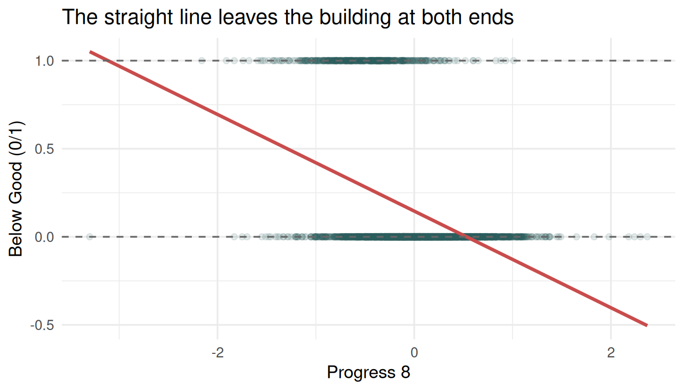
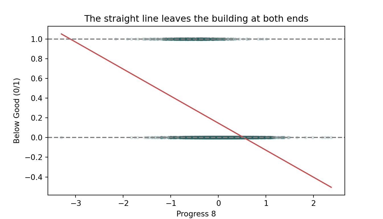
The model’s lowest fitted value is about -0.50. It is telling us that a school with very strong Progress 8 has a minus fifty per cent chance of being rated below Good.

457 schools are given a negative probability. One is given a probability above 1.

Question

A probability of -0.5 is not merely an unlikely event, or a very small chance. What is it? And can you fix this by just rounding the negative predictions up to zero? Write down one reason why that patch would be dishonest before you read on.

Task 2 - See it

Numbers are easy to shrug at. Plot it.

Code

ggplot(model_data, aes(x = P8MEA, y = below_good)) +
  geom_point(alpha = 0.12, colour = "#2E6260") +
  geom_smooth(method = "lm", se = FALSE, colour = "#C94C4C") +
  geom_hline(yintercept = c(0, 1), linetype = "dashed", colour = "grey40") +
  labs(x = "Progress 8", y = "Below Good (0/1)",
       title = "The straight line leaves the building at both ends") +
  theme_minimal(base_size = 13)

Code

import matplotlib.pyplot as plt

fig, ax = plt.subplots(figsize=(7, 4))
ax.scatter(model_data["P8MEA"], model_data["below_good"], alpha=0.12,
           color="#2E6260", s=12)
xs = np.linspace(model_data["P8MEA"].min(), model_data["P8MEA"].max(), 100)
ax.plot(xs, lpm.params["Intercept"] + lpm.params["P8MEA"] * xs, color="#C94C4C")
ax.axhline(0, ls="--", color="grey"); ax.axhline(1, ls="--", color="grey")
ax.set_xlabel("Progress 8"); ax.set_ylabel("Below Good (0/1)")
ax.set_title("The straight line leaves the building at both ends")
plt.show()

The dashed lines at 0 and 1 are the only values the outcome can actually take. The red line crosses both of them and keeps going, because that is what straight lines do. Nothing in lm() knows that probabilities stop.

Part 2: Your first logistic regression

Task 3 - Fit it

The fix is to stop modelling the probability directly, and model the log-odds of it instead - a quantity that is perfectly happy running from minus infinity to plus infinity. That is the link function, and in R and Python it is one argument.

Code

logit1 <- glm(below_good ~ P8MEA, data = model_data, family = binomial)

summary(logit1)


Call:
glm(formula = below_good ~ P8MEA, family = binomial, data = model_data)

Coefficients:
            Estimate Std. Error z value Pr(>|z|)    
(Intercept) -2.32354    0.07386  -31.46   <2e-16 ***
P8MEA       -2.69867    0.13673  -19.74   <2e-16 ***
---
Signif. codes:  0 '***' 0.001 '**' 0.01 '*' 0.05 '.' 0.1 ' ' 1

(Dispersion parameter for binomial family taken to be 1)

    Null deviance: 2678.2  on 3169  degrees of freedom
Residual deviance: 2117.2  on 3168  degrees of freedom
AIC: 2121.2

Number of Fisher Scoring iterations: 6

Code

import statsmodels.api as sm

logit1 = smf.glm("below_good ~ P8MEA", data=model_data,
                 family=sm.families.Binomial()).fit()

print(logit1.summary())

                 Generalized Linear Model Regression Results                  
==============================================================================
Dep. Variable:             below_good   No. Observations:                 3170
Model:                            GLM   Df Residuals:                     3168
Model Family:                Binomial   Df Model:                            1
Link Function:                  Logit   Scale:                          1.0000
Method:                          IRLS   Log-Likelihood:                -1058.6
Date:                Mon, 26 Oct 2026   Deviance:                       2117.2
Time:                        17:12:18   Pearson chi2:                 3.85e+03
No. Iterations:                     6   Pseudo R-squ. (CS):             0.1622
Covariance Type:            nonrobust                                         
==============================================================================
                 coef    std err          z      P>|z|      [0.025      0.975]
------------------------------------------------------------------------------
Intercept     -2.3235      0.074    -31.460      0.000      -2.468      -2.179
P8MEA         -2.6987      0.137    -19.738      0.000      -2.967      -2.431
==============================================================================

Both languages give you an intercept of -2.3235 and a Progress 8 coefficient of -2.6987. Check that yours match before going on.

What changed, and what didn’t

glm(..., family = binomial) instead of lm(...). That is the whole difference in the code. Everything you learned about reading a summary() table - estimates, standard errors, p-values, which predictors earn their place - still applies. What has changed is what the estimates mean, and that is the next two tasks.

Task 4 - The recipe for reading a coefficient

Those coefficients are on the log-odds scale, and nobody thinks in log-odds. The recipe is three steps, and you will use it for the rest of your life:

The recipe

Exponentiate the coefficient. exp(coef) turns a log-odds difference into an odds ratio.
The odds ratio is the multiplier for a one-unit increase in that predictor.
Say it out loud. Above 1 means the odds go up; below 1 means they go down.

Code

exp(coef(logit1))

(Intercept)       P8MEA 
 0.09792662  0.06729478

Code

print(np.exp(logit1.params))

Intercept    0.097927
P8MEA        0.067295
dtype: float64

You should get 0.0979 for the intercept and 0.0673 for Progress 8.

Step 3 is the one that is actually hard, and the one the assessment will ask you for. Here is the Progress 8 one written out:

Every one-point increase in Progress 8 multiplies a school’s odds of being rated below Good by 0.067 - that is, it cuts them to about a fifteenth.

Question

Write the same sentence for the intercept. Two warnings. First, Progress 8 is already centred so that 0 is the national average, which makes the intercept meaningful here - it is the odds for an average school. Second, check it against the data: of the 283 schools within 0.05 of a Progress 8 of zero, what fraction really are below Good? You should find about 6%, where the model puts them at 8.9%. The model is not obliged to match the local average - it is fitting one smooth curve across the whole range, and this is where you see the price of that. Is it a price worth paying?

Task 5 - And back to a probability

Odds are not probabilities, and your reader will want a probability. Going back is one line, and you never have to do it by hand.

Code

new_schools <- data.frame(P8MEA = c(-1, -0.5, 0, 0.5, 1))
new_schools$prob <- predict(logit1, newdata = new_schools, type = "response")
new_schools

  P8MEA        prob
1  -1.0 0.592699378
2  -0.5 0.274044036
3   0.0 0.089192317
4   0.5 0.024774032
5   1.0 0.006546807

Code

new_schools = pd.DataFrame({"P8MEA": [-1, -0.5, 0, 0.5, 1]})
new_schools["prob"] = logit1.predict(new_schools)
print(new_schools)

   P8MEA      prob
0   -1.0  0.592699
1   -0.5  0.274044
2    0.0  0.089192
3    0.5  0.024774
4    1.0  0.006547

Question

type = "response" in R, and plain .predict() in Python, both give you a probability. Look at the five numbers. Are they equally spaced? The Progress 8 values are. Why aren’t the probabilities - and is that a bug or the entire point of what we did in Task 3?

Part 3: More than one predictor

Task 6 - The full model, and the split

Two things happen at once here, and it is worth being clear about why.

First, we add predictors. Second - and this is new - we stop fitting to all the data. From here on the model is fitted on 70% of schools and judged on the 30% it has never seen. Everything in Part 5 depends on that separation, so we do it before we fit rather than bolting it on afterwards.

Why bother — remember the wiggly red line

The lecture showed two models fitted to fifteen points: a sensible curve, and one forced through every single point. The second had an average error of 0.00 on the data it was fitted to, and was the worse of the two on fifteen points it had never seen.

That is overfitting, and it is why a model’s performance on its own training data is not evidence. You can always improve that number by adding terms. The only honest test is data the model has never seen - which is what the next two lines create.

Code

# Deterministic split on sorted row position - identical in R and Python.
# Note the - 1: R counts rows from 1 and Python from 0, and without it the
# two languages would quietly select different schools.
idx   <- seq_len(nrow(model_data)) - 1
test  <- model_data[idx %% 10 <  3, ]
train <- model_data[idx %% 10 >= 3, ]

c(train = nrow(train), test = nrow(test))

train  test 
 2219   951

Code

logit_full <- glm(below_good ~ P8MEA + PTFSM6CLA1A + PERCTOT +
                    PPERSABS10 + log(TPUP) + PTPRIORHI,
                  data = train, family = binomial)

summary(logit_full)


Call:
glm(formula = below_good ~ P8MEA + PTFSM6CLA1A + PERCTOT + PPERSABS10 + 
    log(TPUP) + PTPRIORHI, family = binomial, data = train)

Coefficients:
             Estimate Std. Error z value Pr(>|z|)    
(Intercept) -4.737563   0.988917  -4.791 1.66e-06 ***
P8MEA       -2.265192   0.217525 -10.413  < 2e-16 ***
PTFSM6CLA1A -0.018562   0.006179  -3.004  0.00266 ** 
PERCTOT      0.200477   0.077634   2.582  0.00981 ** 
PPERSABS10   0.003247   0.024202   0.134  0.89327    
log(TPUP)    0.228647   0.173850   1.315  0.18844    
PTPRIORHI   -0.010208   0.009811  -1.040  0.29812    
---
Signif. codes:  0 '***' 0.001 '**' 0.01 '*' 0.05 '.' 0.1 ' ' 1

(Dispersion parameter for binomial family taken to be 1)

    Null deviance: 1934.5  on 2218  degrees of freedom
Residual deviance: 1467.2  on 2212  degrees of freedom
AIC: 1481.2

Number of Fisher Scoring iterations: 6

Code

idx   = np.arange(len(model_data))
test  = model_data[idx % 10 <  3].copy()
train = model_data[idx % 10 >= 3].copy()

print({"train": len(train), "test": len(test)})

{'train': 2219, 'test': 951}

Code

logit_full = smf.glm(
    "below_good ~ P8MEA + PTFSM6CLA1A + PERCTOT + PPERSABS10 "
    "+ np.log(TPUP) + PTPRIORHI",
    data=train, family=sm.families.Binomial()).fit()

print(logit_full.summary())

                 Generalized Linear Model Regression Results                  
==============================================================================
Dep. Variable:             below_good   No. Observations:                 2219
Model:                            GLM   Df Residuals:                     2212
Model Family:                Binomial   Df Model:                            6
Link Function:                  Logit   Scale:                          1.0000
Method:                          IRLS   Log-Likelihood:                -733.58
Date:                Mon, 26 Oct 2026   Deviance:                       1467.2
Time:                        17:12:18   Pearson chi2:                 2.75e+03
No. Iterations:                     7   Pseudo R-squ. (CS):             0.1899
Covariance Type:            nonrobust                                         
================================================================================
                   coef    std err          z      P>|z|      [0.025      0.975]
--------------------------------------------------------------------------------
Intercept       -4.7376      0.989     -4.791      0.000      -6.676      -2.799
P8MEA           -2.2652      0.218    -10.413      0.000      -2.692      -1.839
PTFSM6CLA1A     -0.0186      0.006     -3.004      0.003      -0.031      -0.006
PERCTOT          0.2005      0.078      2.582      0.010       0.048       0.353
PPERSABS10       0.0032      0.024      0.134      0.893      -0.044       0.051
np.log(TPUP)     0.2286      0.174      1.315      0.188      -0.112       0.569
PTPRIORHI       -0.0102      0.010     -1.040      0.298      -0.029       0.009
================================================================================

You should have 2,219 training and 951 test schools, and an intercept of -4.7376.

Your numbers will not match the lecture’s — and that is correct

The lecture split the schools with set.seed(42) and sample(). We split on sorted row position instead, for the reason given at the top: R’s and Python’s random number generators will never agree with each other.

Both splits take 70/30 of the same 3,170 schools, so both give 2,219 and 951. But they are a different 951 schools — so every test-set figure from here on differs a little from the lecture’s:

	Lecture	Here
Test-set accuracy	86.2%	86.9%
Majority-class baseline	85.3%	86.9%
AUC	0.818	0.812

Do not go hunting for a bug. The conclusion is the same in both, and here it is even clearer: in the lecture the model beat the baseline by 0.9 points, and on this split it does not beat it at all.

Task 7 - Say all six out loud

Same recipe as Task 4, applied six times.

Code

round(exp(coef(logit_full)), 4)

(Intercept)       P8MEA PTFSM6CLA1A     PERCTOT  PPERSABS10   log(TPUP) 
     0.0088      0.1038      0.9816      1.2220      1.0033      1.2569 
  PTPRIORHI 
     0.9898

Code

print(np.exp(logit_full.params).round(4))

Intercept       0.0088
P8MEA           0.1038
PTFSM6CLA1A     0.9816
PERCTOT         1.2220
PPERSABS10      1.0033
np.log(TPUP)    1.2569
PTPRIORHI       0.9898
dtype: float64

Question - this is the exercise, not the code

Write one plain-English sentence per predictor. Then answer two harder questions:

PERCTOT (overall absence) has an odds ratio above 1, and PTFSM6CLA1A (free school meals) has one just below. Does that mean absence matters and poverty does not? What else changed when you moved from one predictor to six?
The intercept is now the odds for a school with Progress 8 of zero, zero free school meals, zero absence, zero prior-high-attainers and a cohort of one pupil - because log(TPUP) is 0 when TPUP is 1. How many such schools exist? What does that tell you about quoting the intercept in a write-up?

Task 8 - Centre the predictors, and get an intercept worth quoting

Task 7 left you with a useless intercept: the odds for a school with a cohort of one pupil, no absence and no disadvantaged pupils. No such school exists.

There is a standard fix. Subtract each predictor’s mean from itself, so that zero stops meaning none and starts meaning average. Progress 8 already arrives this way - that is why it behaved sensibly in Task 3.

Code

train_c <- train |>
  mutate(log_TPUP = log(TPUP),
         across(c(P8MEA, PTFSM6CLA1A, PERCTOT, PPERSABS10, log_TPUP, PTPRIORHI),
                ~ .x - mean(.x), .names = "c_{.col}"))

logit_centred <- glm(below_good ~ c_P8MEA + c_PTFSM6CLA1A + c_PERCTOT +
                       c_PPERSABS10 + c_log_TPUP + c_PTPRIORHI,
                     data = train_c, family = binomial)

# the intercept, three ways
c(log_odds = coef(logit_centred)[[1]],
  odds     = exp(coef(logit_centred)[[1]]),
  prob     = plogis(coef(logit_centred)[[1]]))

   log_odds        odds        prob 
-2.31740588  0.09852885  0.08969164

Code

train_c = train.copy()
train_c["log_TPUP"] = np.log(train_c["TPUP"])
for v in ["P8MEA", "PTFSM6CLA1A", "PERCTOT", "PPERSABS10", "log_TPUP", "PTPRIORHI"]:
    train_c["c_" + v] = train_c[v] - train_c[v].mean()

logit_centred = smf.glm(
    "below_good ~ c_P8MEA + c_PTFSM6CLA1A + c_PERCTOT + c_PPERSABS10 "
    "+ c_log_TPUP + c_PTPRIORHI",
    data=train_c, family=sm.families.Binomial()).fit()

b0 = logit_centred.params["Intercept"]
print({"log_odds": round(b0, 4),
       "odds": round(np.exp(b0), 4),
       "prob": round(1 / (1 + np.exp(-b0)), 4)})

{'log_odds': np.float64(-2.3174), 'odds': np.float64(0.0985), 'prob': np.float64(0.0897)}

Compare the two intercepts

	Intercept	$e^{\beta_0}$ (odds)	as a probability
Task 6 model, uncentred	−4.7376	0.0088	0.9%
Centred	−2.3174	0.0985	9.0%

The first describes a school that does not exist. The second describes a school at the average of every predictor - and that is a sentence you can put in a report.

Questions

Compare the other six coefficients with the ones from Task 7. They should be identical - and so should the deviance, the AIC and every pseudo-R². Check that they are. If centring changes none of those, what exactly has it changed, and why was it worth doing?
Write the sentence. “A school at the national average on every one of these measures has a ___ chance of being rated below Good.”
The awkward one. 15.8% of the training schools really are below Good, but the centred intercept says an average school has a 9.0% chance. Those are not the same number and neither is wrong. Why not? (Hint: the model is linear in log-odds, not in probability - so the probability at the average school is not the average of the probabilities. You met this in Week 1 as the difference between the mean of the logs and the log of the mean.)
Centring is not the only option. What would you subtract instead if you wanted the intercept to describe a specific, real school - say, a median-sized school in your own local authority?

Part 4: Does the model fit?

Task 9 - Deviance, AIC and the pseudo-R-squareds

There is no R-squared here, because there are no residuals in the sense OLS means. What we have instead is a set of numbers built on the likelihood - how surprised the model is by the data it saw.

Every one of these is already sitting in the output you printed at Task 6. The point of this task is to find them there, not to compute them afresh.

Code

logLik(logit_full)

'log Lik.' -733.5766 (df=7)

Code

logit_full$null.deviance   # a model with the intercept only

[1] 1934.454

Code

logit_full$deviance        # our model

[1] 1467.153

Code

AIC(logit_full)

[1] 1481.153

Code

# The pseudo-R-squareds are not in base R
performance::r2_coxsnell(logit_full)

Cox & Snell's R2 
       0.1898946

Code

performance::r2_nagelkerke(logit_full)

Nagelkerke's R2 
      0.3263978

Code

print(logit_full.llf)          # log-likelihood

-733.576641893507

Code

print(logit_full.null_deviance)

1934.4544835675365

Code

print(logit_full.deviance)

1467.153283787014

Code

print(logit_full.aic)

1481.153283787014

Code

# statsmodels has no built-in pseudo-R2 for GLM, so compute them directly
n   = logit_full.nobs
cs  = 1 - np.exp((logit_full.llnull - logit_full.llf) * 2 / n)
nag = cs / (1 - np.exp(2 * logit_full.llnull / n))
print({"Cox & Snell": round(cs, 4), "Nagelkerke": round(nag, 4)})

{'Cox & Snell': np.float64(0.1899), 'Nagelkerke': np.float64(0.3264)}

Python trap — .prsquared is not the number you just computed

smf.glm() has no .prsquared attribute. smf.logit() does, and it is very tempting to reach for it instead of writing those two lines out.

It is McFadden’s pseudo-R², which is a different measure built a different way. Fit this model both ways and compare:

lg = smf.logit("below_good ~ P8MEA + PTFSM6CLA1A + PERCTOT + PPERSABS10 "
               "+ np.log(TPUP) + PTPRIORHI", data=train).fit(disp=0)
print(lg.prsquared)

You should get 0.2416, against the 0.3264 Nagelkerke you computed above. Same data, same fit, two numbers with the same nickname. Whichever you report, name it.

R users are not immune: performance::r2_mcfadden() sits right next to r2_nagelkerke() and will give you the same 0.2416.

How to read them

Null deviance vs residual deviance. The first is how badly an intercept-only model does; the second is how badly ours does. The drop between them is what the predictors bought you.
AIC is the log-likelihood with a fine for each extra parameter. It is only meaningful compared with another model on the same data - an AIC on its own means nothing at all.
Cox & Snell cannot reach 1, even for a perfect model. Nagelkerke rescales it so that it can. Neither one is “the proportion of variance explained”, whatever your software calls it.

Question

Drop PTPRIORHI and refit. Does AIC go up or down? Now drop P8MEA instead. Which of the two was carrying the model - and does the answer surprise you, given the p-values?

Part 5: Does it make good decisions?

This part is not just about logistic regression

Holding data back, comparing against a baseline, and separating fit from prediction apply to every model you will ever build, including the OLS and multilevel models of the past three weeks. What is specific to today is only the scoreboard - accuracy, confusion matrices and AUC need a categorical outcome to be defined at all.

Task 10 - Predict, and compare with doing nothing

The model does not hand back a yes or a no. For each school it hands back a probability, so before counting anything, watch what the 0.5 cut-off does to four individual schools.

10a - Four schools, one at a time

Code

p_below <- predict(logit_full, newdata = test, type = "response")

flag <- p_below > 0.5
act  <- test$below_good == 1

# one real school nearest each of four illustrative probabilities
pick <- function(sel, target) {
  i <- which(sel); i[which.min(abs(p_below[i] - target))]
}
idx <- c(pick(!flag & !act, 0.03), pick(flag &  act, 0.70),
         pick(!flag &  act, 0.30), pick(flag & !act, 0.60))

data.frame(
  school      = c("A", "B", "C", "D"),
  probability = round(p_below[idx], 2),
  above_0.5   = ifelse(p_below[idx] > 0.5, "yes", "no"),
  predicted   = ifelse(p_below[idx] > 0.5, "Below Good", "Good or better"),
  actual      = ifelse(act[idx], "Below Good", "Good or better"),
  right       = ifelse((p_below[idx] > 0.5) == act[idx], "yes", "no"),
  row.names   = NULL
)

  school probability above_0.5      predicted         actual right
1      A        0.03        no Good or better Good or better   yes
2      B        0.72       yes     Below Good     Below Good   yes
3      C        0.30        no Good or better     Below Good    no
4      D        0.60       yes     Below Good Good or better    no

Code

p_below = logit_full.predict(test)

flag = p_below > 0.5
act  = test["below_good"] == 1

def pick(sel, target):
    return (p_below[sel] - target).abs().idxmin()

idx = [pick(~flag & ~act, 0.03), pick(flag &  act, 0.70),
       pick(~flag &  act, 0.30), pick(flag & ~act, 0.60)]

print(pd.DataFrame({
    "school":      ["A", "B", "C", "D"],
    "probability": p_below[idx].round(2).values,
    "above_0.5":   np.where(p_below[idx] > 0.5, "yes", "no"),
    "predicted":   np.where(p_below[idx] > 0.5, "Below Good", "Good or better"),
    "actual":      np.where(act[idx], "Below Good", "Good or better"),
    "right":       np.where((p_below[idx] > 0.5) == act[idx], "yes", "no"),
}))

  school  probability above_0.5       predicted          actual right
0      A         0.03        no  Good or better  Good or better   yes
1      B         0.72       yes      Below Good      Below Good   yes
2      C         0.30        no  Good or better      Below Good    no
3      D         0.60       yes      Below Good  Good or better    no

What just happened

C was missed and D was a false alarm. Each school is judged on its own probability - the cut-off simply sorts them either side of the line, one school at a time.

So 0.5 is not “half the time”. Applied to all 951 test schools it flags 48 of them, not 476.

10b - Now count them all

Here is the whole trap in one step. Count how often you were right, and then count how often you would have been right by not building a model at all - by simply saying “not below Good” to every school.

Code

p_below  <- predict(logit_full, newdata = test, type = "response")

accuracy <- mean((p_below > 0.5) == test$below_good)
baseline <- max(mean(test$below_good), 1 - mean(test$below_good))

c(accuracy = round(accuracy, 4), baseline = round(baseline, 4))

accuracy baseline 
  0.8686   0.8686

Code

p_below = logit_full.predict(test)

accuracy = ((p_below > 0.5).astype(int) == test["below_good"]).mean()
baseline = max(test["below_good"].mean(), 1 - test["below_good"].mean())

print({"accuracy": round(accuracy, 4), "baseline": round(baseline, 4)})

{'accuracy': np.float64(0.8686), 'baseline': np.float64(0.8686)}

Stop here and look at those two numbers

They are the same: 0.8686 and 0.8686. Six predictors, a proper model, a clean train/test split - and it classifies schools exactly as well as a rule that ignores the data entirely.

This is not a mistake in your code. It is what the 15% was always going to do to us, and it is the most useful result in this practical.

10c - That baseline is a model you have already fitted

We worked the baseline out arithmetically - what share would I get right by always guessing the commoner answer? But it is also a model: an intercept and nothing else. R and statsmodels will fit it for you.

Code

null_mod <- glm(below_good ~ 1, data = train, family = binomial)
p_null   <- predict(null_mod, newdata = test, type = "response")

c(distinct_predictions = length(unique(round(p_null, 10))),
  it_predicts          = round(unique(p_null)[[1]], 4),
  its_accuracy         = round(mean((p_null > 0.5) == test$below_good), 4),
  our_baseline         = round(baseline, 4))

distinct_predictions          it_predicts         its_accuracy 
              1.0000               0.1577               0.8686 
        our_baseline 
              0.8686

Code

null_mod = smf.glm("below_good ~ 1", data=train,
                   family=sm.families.Binomial()).fit()
p_null = null_mod.predict(test)

print({"distinct_predictions": p_null.round(10).nunique(),
       "it_predicts":  round(p_null.iloc[0], 4),
       "its_accuracy": round(((p_null > 0.5).astype(int) == test["below_good"]).mean(), 4),
       "our_baseline": round(baseline, 4)})

{'distinct_predictions': 1, 'it_predicts': np.float64(0.1577), 'its_accuracy': np.float64(0.8686), 'our_baseline': np.float64(0.8686)}

Why they are the same number

The null model makes one distinct prediction - 0.1577, the share of training schools below Good - for every school in the test set. That is below 0.5, so thresholding sends every school to “Good or better”, which is exactly the always-say-no rule. Hence the identical accuracy.

Now compare null_mod$deviance with the null_deviance you printed back in Task 9. They are the same number, because that is what null deviance is: the deviance of this model. R has been fitting it for you every time you call glm() - you have just never looked at it.

Question

Would the two still agree if below-Good schools were the majority - say 60% of them? Work out what the null model would predict, what thresholding at 0.5 would then do, and what the majority-class baseline would be.

Task 11 - The confusion matrix shows you why

Accuracy is one number squashed out of four, and the four are more honest.

Code

table(Actual    = ifelse(test$below_good == 1, "Below Good", "Good or better"),
      Predicted = ifelse(p_below > 0.5,        "Below Good", "Good or better"))

                Predicted
Actual           Below Good Good or better
  Below Good             24            101
  Good or better         24            802

Code

print(pd.crosstab(
    test["below_good"].map({1: "Below Good", 0: "Good or better"}),
    pd.Series(np.where(p_below > 0.5, "Below Good", "Good or better"),
              index=test.index),
    rownames=["Actual"], colnames=["Predicted"]))

Predicted       Below Good  Good or better
Actual                                    
Below Good              24             101
Good or better          24             802

Of the 125 schools that really are below Good, the model flags 24 and misses 101. It also raises 24 false alarms. The gains and the losses cancel exactly, which is why accuracy came out identical to the baseline.

Question

A school improvement team has to decide where to send inspectors. Which of the four cells in that table costs them most? Does accuracy weight it that way?

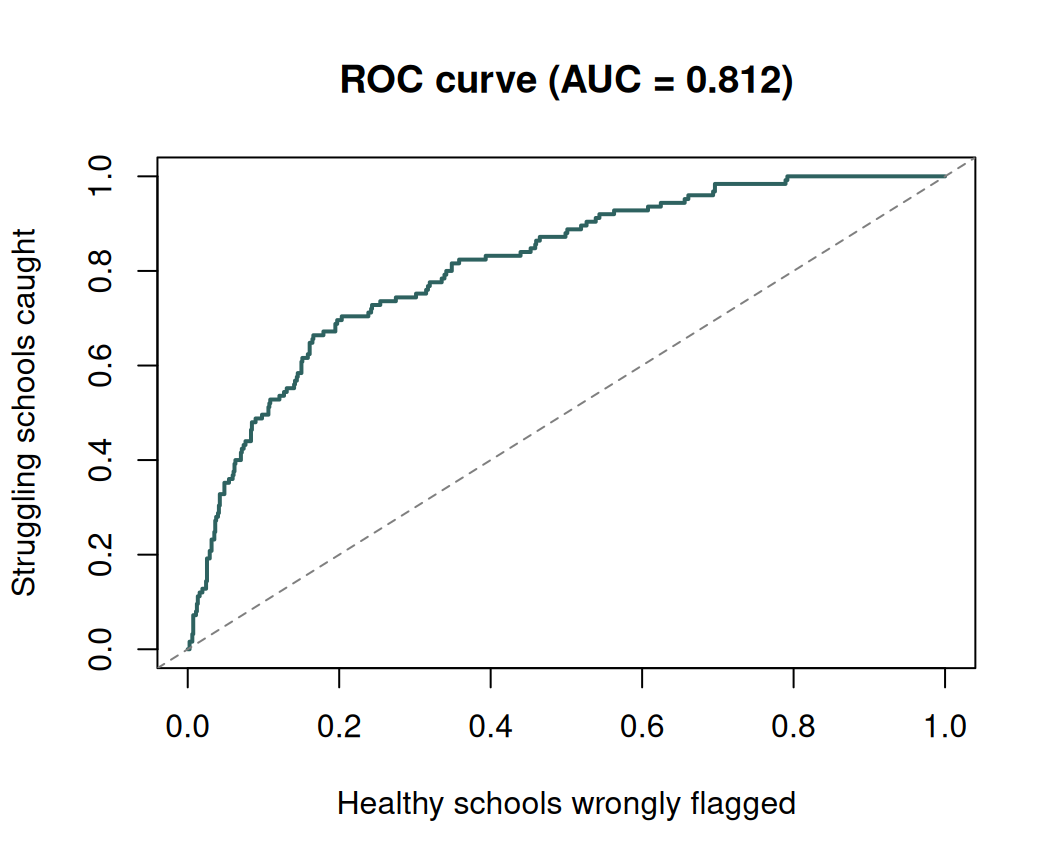
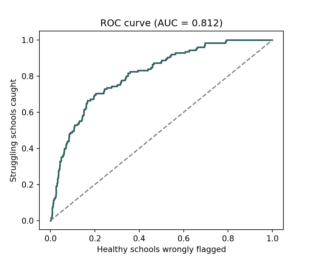
Task 12 - ROC and AUC: judge the ranking instead

Everything above hung on the cut-off of 0.5, and nothing made 0.5 right. So ask a question that does not depend on it at all: does the model put schools in the right order?

ROC stands for Receiver Operating Characteristic, a name inherited from WWII radar operators and one that tells you nothing useful. AUC is the Area Under the Curve.

Code

roc <- performance::performance_roc(logit_full, new_data = test)
auc <- bayestestR::area_under_curve(roc$Specificity, roc$Sensitivity)
auc

[1] 0.8118063

Code

plot(roc$Specificity, roc$Sensitivity, type = "l", lwd = 2, col = "#2E6260",
     xlab = "Healthy schools wrongly flagged",
     ylab = "Struggling schools caught",
     main = paste0("ROC curve (AUC = ", round(auc, 3), ")"))
abline(0, 1, lty = 2, col = "grey50")

Code

from sklearn.metrics import roc_curve, roc_auc_score

fpr, tpr, thresholds = roc_curve(test["below_good"], p_below)
auc = roc_auc_score(test["below_good"], p_below)
print(round(auc, 4))

0.8118

Code

fig, ax = plt.subplots(figsize=(5.5, 4.5))
ax.plot(fpr, tpr, lw=2, color="#2E6260")
ax.plot([0, 1], [0, 1], ls="--", color="grey")
ax.set_xlabel("Healthy schools wrongly flagged")
ax.set_ylabel("Struggling schools caught")
ax.set_title(f"ROC curve (AUC = {auc:.3f})")
plt.show()

AUC comes out at 0.812. Read it like this:

Pick one school that really is below Good and one that really is not. The model gives the struggling one the higher predicted probability of being below Good 81% of the time.

That “predicted probability” is the model’s own output - the 0-to-1 number you called p_below - and not Progress 8 or any other predictor.

Both things are true at once

The model classifies no better than doing nothing, and it ranks schools well. There is no contradiction. We were reading a good ranking at a cut-off that threw the ranking away.

Task 13 - Now choose a cut-off

Only now that you know the model ranks sensibly is the cut-off a sensible question - and it is a policy question, not a statistical one.

Code

thresholds <- c(0.5, 0.3, 0.2, 0.1)

data.frame(
  cut_off      = thresholds,
  caught       = sapply(thresholds, function(t) sum(p_below >  t & test$below_good == 1)),
  missed       = sapply(thresholds, function(t) sum(p_below <= t & test$below_good == 1)),
  false_alarms = sapply(thresholds, function(t) sum(p_below >  t & test$below_good == 0))
)

  cut_off caught missed false_alarms
1     0.5     24    101           24
2     0.3     60     65           73
3     0.2     83     42          147
4     0.1    104     21          328

Code

rows = []
for t in [0.5, 0.3, 0.2, 0.1]:
    flag = p_below > t
    rows.append({"cut_off": t,
                 "caught": int((flag & (test.below_good == 1)).sum()),
                 "missed": int((~flag & (test.below_good == 1)).sum()),
                 "false_alarms": int((flag & (test.below_good == 0)).sum())})
print(pd.DataFrame(rows))

   cut_off  caught  missed  false_alarms
0      0.5      24     101            24
1      0.3      60      65            73
2      0.2      83      42           147
3      0.1     104      21           328

Question - and it is the one that matters

Pick a cut-off and defend it in two sentences, naming who bears the cost of the misses and who bears the cost of the false alarms. There is no correct answer here, and that is the point: AUC told you the curve was worth picking from, but it cannot tell you where on it to sit.

Part 6: Extensions

Two routes out of here. Pick one - they are both a solid hour - and come back for the other if you have time. Extension A connects today to last week; Extension B connects today to the rest of the GLM family.

Extension A - Take ROC back to the multilevel model

Last week you fitted a linear mixed effects model with local authority as a grouping variable. The obvious question is whether you can put a ROC curve on it.

Read this before you try - the honest answer is ‘not directly’

You cannot run a ROC curve on last week’s model as it stands. ROC and AUC need a binary outcome: the curve is built by counting how many of the 1s you caught against how many of the 0s you wrongly flagged, and if the outcome is a continuous Attainment 8 score there are no 1s and 0s to count.

This is not a technicality to work around. It is the same point as the callout at the top of Part 5: holding data back and comparing against a baseline transfer to any model, but the scoreboard does not.

So the interesting version of this extension is not “ROC the old model”. It is: keep the grouping structure, change the outcome to a binary one, and you get a model that is both of the last two weeks at once - a generalised linear mixed model.

A1 - Fit a mixed-effects logistic regression

A random intercept for local authority, on top of the logistic regression you already have. In R this is glmer() - lmer() with a family argument, exactly the way glm() was lm() with a family argument.

Code

library(lme4)

glmm <- glmer(below_good ~ P8MEA + PTFSM6CLA1A + PERCTOT + (1 | LANAME),
              data = train, family = binomial)

summary(glmm)

Generalized linear mixed model fit by maximum likelihood (Laplace
  Approximation) [glmerMod]
 Family: binomial  ( logit )
Formula: below_good ~ P8MEA + PTFSM6CLA1A + PERCTOT + (1 | LANAME)
   Data: train

      AIC       BIC    logLik -2*log(L)  df.resid 
   1473.7    1502.2    -731.8    1463.7      2214 

Scaled residuals: 
    Min      1Q  Median      3Q     Max 
-8.1764 -0.3804 -0.2285 -0.1087 12.4463 

Random effects:
 Groups Name        Variance Std.Dev.
 LANAME (Intercept) 0.1881   0.4337  
Number of obs: 2219, groups:  LANAME, 151

Fixed effects:
            Estimate Std. Error z value Pr(>|z|)    
(Intercept) -4.05177    0.36170 -11.202  < 2e-16 ***
P8MEA       -2.27607    0.22118 -10.291  < 2e-16 ***
PTFSM6CLA1A -0.01819    0.00640  -2.842  0.00448 ** 
PERCTOT      0.23100    0.03827   6.036 1.58e-09 ***
---
Signif. codes:  0 '***' 0.001 '**' 0.01 '*' 0.05 '.' 0.1 ' ' 1

Correlation of Fixed Effects:
            (Intr) P8MEA  PTFSM6
P8MEA       -0.402              
PTFSM6CLA1A -0.112  0.261       
PERCTOT     -0.857  0.430 -0.331

Code

# How much do local authorities differ, once the predictors are accounted for?
VarCorr(glmm)

 Groups Name        Std.Dev.
 LANAME (Intercept) 0.43372

Code

from statsmodels.genmod.bayes_mixed_glm import BinomialBayesMixedGLM

glmm = BinomialBayesMixedGLM.from_formula(
    "below_good ~ P8MEA + PTFSM6CLA1A + PERCTOT",
    {"LANAME": "0 + C(LANAME)"},
    train).fit_vb(verbose=False)

print(glmm.summary())

                Binomial Mixed GLM Results
==========================================================
            Type Post. Mean Post. SD   SD  SD (LB) SD (UB)
----------------------------------------------------------
Intercept      M    -3.9631   0.0672                      
P8MEA          M    -2.2934   0.1260                      
PTFSM6CLA1A    M    -0.0185   0.0020                      
PERCTOT        M     0.2231   0.0062                      
LANAME         V    -0.8041   0.0576 0.447   0.399   0.502
==========================================================
Parameter types are mean structure (M) and variance
structure (V)
Variance parameters are modeled as log standard deviations

A real difference between the two languages

This is the one place in the practical where the tabs do not give you the same numbers, and you should know why.

glmer() fits by maximum likelihood. statsmodels’ BinomialBayesMixedGLM fits by variational Bayes - a different estimator of a differently specified model - so the coefficients land close but not identical, and the summary reports posterior means rather than estimates and standard errors. The local authority standard deviation comes out at about 0.43 from glmer() and 0.45 from statsmodels - close enough that the conclusion is the same either way, which is the point.

Python’s mixed-model support is genuinely thinner than R’s - and you will feel it in A2, where there is no predict() that takes new data and the random effects, so we rebuild the linear predictor by hand. If you need mixed models seriously in Python, pymer4 (which calls lme4 underneath) and bambi are the usual answers.

A2 - Did the grouping actually help the ranking?

Here is where today’s scoreboard earns its keep. Fit the same model without the random intercept, predict both on the held-out schools, and compare AUC.

Code

flat <- glm(below_good ~ P8MEA + PTFSM6CLA1A + PERCTOT,
            data = train, family = binomial)

auc_of <- function(scores, actual) {
  r  <- rank(scores)
  n1 <- sum(actual == 1); n0 <- sum(actual == 0)
  (sum(r[actual == 1]) - n1 * (n1 + 1) / 2) / (n1 * n0)
}

p_glmm <- predict(glmm, newdata = test, type = "response",
                  allow.new.levels = TRUE)
p_flat <- predict(flat, newdata = test, type = "response")

c(mixed = round(auc_of(p_glmm, test$below_good), 4),
  flat  = round(auc_of(p_flat, test$below_good), 4))

 mixed   flat 
0.8149 0.8121

Code

import patsy
from sklearn.metrics import roc_auc_score

# statsmodels has no predict() that takes new data *and* the random effects,
# so we rebuild the linear predictor by hand: fixed part + this school's
# local-authority effect.
X_test = patsy.dmatrix("P8MEA + PTFSM6CLA1A + PERCTOT", test, return_type="dataframe")
eta    = X_test.values @ glmm.fe_mean

re_mean = glmm.random_effects()["Mean"]
re_map  = {k.split("[")[1].rstrip("]"): v for k, v in re_mean.items()}
# .fillna(0) is this language's allow.new.levels: an unseen authority
# simply gets the average intercept
eta += test["LANAME"].map(re_map).fillna(0.0).values

p_glmm = 1 / (1 + np.exp(-eta))

flat   = smf.glm("below_good ~ P8MEA + PTFSM6CLA1A + PERCTOT",
                 data=train, family=sm.families.Binomial()).fit()
p_flat = flat.predict(test)

print({"mixed": round(roc_auc_score(test["below_good"], p_glmm), 4),
       "flat":  round(roc_auc_score(test["below_good"], p_flat),  4)})

{'mixed': 0.8154, 'flat': 0.8121}

The two languages will not quite agree, and that is expected

R gets a mixed-model AUC of 0.8149; Python gets about 0.8154. The flat models agree exactly, because both are ordinary glm() fits - the difference is entirely in the mixed model, where glmer() maximises the likelihood and statsmodels runs variational Bayes. Close, not identical, and for the same reason the coefficients differed in A1.

Question - and do not assume the answer

The mixed model gets 0.8149; the flat one gets 0.8121. Modelling 151 local authorities bought you 0.003 of AUC.

Was the random intercept worth it? Answer for an explanatory aim and for a predictive aim separately - the honest answers differ.
allow.new.levels = TRUE - and .fillna(0) in the Python - is doing something specific when a test-set school sits in a local authority the training set never saw. What? And why does that limit how much a group-level model can ever buy you on held-out data?
The LA standard deviation is 0.43 on the log-odds scale, which is not nothing. How can there be real variation between authorities and almost no gain in ranking?

Extension B - A different family: counts, offsets and the negative binomial

Same recipe, different member of the family. Here the outcome is a count: how many schools in each local authority are rated below Good?

B1 - Build the counts

Code

la <- model_data |>
  group_by(LANAME) |>
  summarise(n_below   = sum(below_good),
            n_schools = n(),
            mean_fsm  = mean(PTFSM6CLA1A),
            mean_abs  = mean(PERCTOT),
            .groups   = "drop") |>
  filter(n_schools >= 5)

nrow(la)

[1] 150

Code

summary(la$n_below)

   Min. 1st Qu.  Median    Mean 3rd Qu.    Max. 
  0.000   1.000   3.000   3.167   4.000  22.000

Code

la = (model_data
      .groupby("LANAME")
      .agg(n_below=("below_good", "sum"),
           n_schools=("below_good", "size"),
           mean_fsm=("PTFSM6CLA1A", "mean"),
           mean_abs=("PERCTOT", "mean"))
      .reset_index())
la = la[la["n_schools"] >= 5]

print(len(la))

Code

print(la["n_below"].describe())

count    150.000000
mean       3.166667
std        3.139736
min        0.000000
25%        1.000000
50%        3.000000
75%        4.000000
max       22.000000
Name: n_below, dtype: float64

B2 - Poisson regression, with an offset

An authority with 60 schools will have more schools below Good than one with 8, for reasons that have nothing to do with poverty or absence. The offset is how you tell the model to work in rates rather than raw counts: it is a predictor whose coefficient is fixed at 1 rather than estimated.

Code

pois <- glm(n_below ~ mean_fsm + mean_abs + offset(log(n_schools)),
            data = la, family = poisson)

summary(pois)


Call:
glm(formula = n_below ~ mean_fsm + mean_abs + offset(log(n_schools)), 
    family = poisson, data = la)

Coefficients:
             Estimate Std. Error z value Pr(>|z|)    
(Intercept) -4.444128   0.442163 -10.051  < 2e-16 ***
mean_fsm    -0.002045   0.005498  -0.372     0.71    
mean_abs     0.279270   0.048094   5.807 6.37e-09 ***
---
Signif. codes:  0 '***' 0.001 '**' 0.01 '*' 0.05 '.' 0.1 ' ' 1

(Dispersion parameter for poisson family taken to be 1)

    Null deviance: 224.29  on 149  degrees of freedom
Residual deviance: 190.24  on 147  degrees of freedom
AIC: 573.49

Number of Fisher Scoring iterations: 5

Code

pois = smf.glm("n_below ~ mean_fsm + mean_abs",
               data=la, family=sm.families.Poisson(),
               offset=np.log(la["n_schools"])).fit()

print(pois.summary())

                 Generalized Linear Model Regression Results                  
==============================================================================
Dep. Variable:                n_below   No. Observations:                  150
Model:                            GLM   Df Residuals:                      147
Model Family:                 Poisson   Df Model:                            2
Link Function:                    Log   Scale:                          1.0000
Method:                          IRLS   Log-Likelihood:                -283.74
Date:                Mon, 26 Oct 2026   Deviance:                       190.24
Time:                        17:12:23   Pearson chi2:                     183.
No. Iterations:                     5   Pseudo R-squ. (CS):             0.2031
Covariance Type:            nonrobust                                         
==============================================================================
                 coef    std err          z      P>|z|      [0.025      0.975]
------------------------------------------------------------------------------
Intercept     -4.4441      0.442    -10.051      0.000      -5.311      -3.578
mean_fsm      -0.0020      0.005     -0.372      0.710      -0.013       0.009
mean_abs       0.2793      0.048      5.807      0.000       0.185       0.374
==============================================================================

Question

Fit it again without the offset and compare the coefficients. Which one changes most, and can you explain why in terms of what the offset was soaking up?

B3 - Is it overdispersed?

The Poisson model assumes the variance equals the mean. That is a strong assumption and it is usually wrong. Check it before you believe any of the standard errors.

Code

sum(residuals(pois, type = "pearson")^2) / df.residual(pois)

[1] 1.247152

Code

print(pois.pearson_chi2 / pois.df_resid)

1.2471515060731997

You should get 1.247. A value of 1 is what Poisson assumes; much above 2 and the Poisson standard errors are badly optimistic. 1.25 is mild.

B4 - Fit the negative binomial anyway, and decide whether it was needed

The negative binomial adds one parameter that lets the variance exceed the mean. Fit it, and then make it earn its place.

Code

nb <- MASS::glm.nb(n_below ~ mean_fsm + mean_abs + offset(log(n_schools)),
                   data = la)

c(poisson_AIC = round(AIC(pois), 1),
  nb_AIC      = round(AIC(nb), 1),
  theta       = round(nb$theta, 2))

poisson_AIC      nb_AIC       theta 
     573.50      572.40       19.72

Code

nb = smf.negativebinomial("n_below ~ mean_fsm + mean_abs",
                          data=la, offset=np.log(la["n_schools"])).fit(disp=0)

print({"poisson_AIC": round(pois.aic, 1),
       "nb_AIC": round(nb.aic, 1),
       "alpha": round(nb.params["alpha"], 4)})

{'poisson_AIC': np.float64(573.5), 'nb_AIC': np.float64(572.4), 'alpha': np.float64(0.0507)}

The result you were probably not expecting

Poisson AIC 573.5, negative binomial AIC 572.4. One AIC point, for a whole extra parameter.

R reports theta = 19.72 and Python reports alpha = 0.0507. They are the same number: alpha is 1/theta. A large theta - equivalently an alpha near zero - means the negative binomial has collapsed back towards the Poisson, because there was barely any extra dispersion for it to model.

The negative binomial was not needed here. That is a perfectly good finding, and far more useful than reaching for the fancier model by reflex. Report the dispersion statistic, report that you checked, and keep the simpler model.

Question

Now go and find a count outcome in the DfE files that is badly overdispersed, and run the same four steps on it. Pupil destinations is a good hunting ground. What would you have got wrong if you had trusted the Poisson standard errors?

Where this goes in your assessment

Three habits from today are worth carrying into the coursework, whatever model you end up fitting:

Look at the outcome before choosing the model. Binary, count, proportion, ordered category and continuous each have a family that fits them. Picking the family is a modelling decision you should justify in a sentence, not a default you fell into.
Never report accuracy without the baseline beside it. Today’s model scored 86.9%, which sounds respectable until you notice that doing nothing also scores 86.9%.
Say what you are for. If you are explaining, judge the model on the data you fitted it to and interpret the coefficients. If you are predicting, hold data back and judge it there. Both are legitimate. Deciding which one you are doing before you start changes what counts as a good model, and a write-up that quietly switches between them is the commonest way to overclaim.