Prof D’s Regression Sessions - Vol 4
Breaking the mould - generalised linear models
Adam Dennett - a.dennett@ucl.ac.uk
Week GLM
CASA0007 Quantitative Methods
Recap
- Over three weeks we built a regression model up from a single scatter plot to a linear mixed effects model with random intercepts and random slopes
- We learned a recipe - understand your data, start simple, add complexity only when it earns its place, and check your assumptions at every step
- Last week we relaxed one particular assumption: that our observations were independent. Schools sit inside local authorities, and that grouping matters
But one thing never changed
- Every single model we have fitted has had a continuous outcome variable
- Attainment 8. Progress 8. Numbers that can take any value, that are roughly bell-shaped, and that happily sit on either side of a straight line
- This choice let us use Ordinary Least Squares throughout - but we know that our data don’t always look like this
- What happens when the thing you want to explain is a yes/no, a category, or a count?
This week’s session aims
- Understand why OLS fails when the outcome is not continuous, and see it fail
- Meet the Generalised Linear Model (GLM) - one framework, three moving parts
- Logistic regression for binary outcomes, then ordinal and multinomial versions for categories
- Poisson regression for counts, offsets for rates, and what to do about overdispersion
- How to judge one when there is no R² - deviance, AIC, the pseudo-R²s, and whether the predictions are actually any use
- Throughout: can we predict a school’s Ofsted rating from everything else we know about it?
Back to Week 1
Remember these?
In week 1 we spent a long time on types of data, and on the distributions that go with them.
| Data type | Example from our data | Distribution |
|---|---|---|
| Real-valued | Attainment 8 | Normal |
| Binary | Is this school single-sex? | Bernoulli / Binomial |
| Count | How many pupils on free school meals? | Poisson |
| Count, overdispersed | … when the variance exceeds the mean | Negative binomial |
| Ordinal | Ofsted rating | (no single answer) |
We then spent three weeks modelling only the first row!
The whole idea of a GLM, in one table
| If your outcome is… | …its distribution is | …the model is |
|---|---|---|
| A continuous number | Normal | OLS - weeks 5, 6, 7 |
| A yes/no | Binomial | Logistic regression |
| A proportion out of a known total | Binomial | Logistic regression |
| An ordered category | - | Ordinal logistic |
| An unordered category | - | Multinomial logistic |
| A count | Poisson | Poisson regression |
| A count that is too variable | Negative binomial | Negative binomial regression |
This is not seven new methods. It is one method, with a slot you fill differently depending on what you are trying to explain.
What actually changes
Every GLM has exactly three pieces. You already know the middle one.
- The random component - what distribution does the outcome follow? (Normal, binomial, Poisson…)
- The linear predictor - \(\beta_0 + \beta_1x_1 + \beta_2x_2 + ...\) . This is identical to everything we have done for three weeks
- The link function - the bit of maths that connects the two, so that a straight line on one scale becomes a sensible prediction on the other
OLS is just the GLM where the distribution is Normal and the link function does nothing at all.
A quick word on \(E[y]\)
With GLMs there is an \(E\) in most of the equations. \(E\) is for expectation, and \(E[y_i]\) reads “the expected value of y for school i”.
- It is essentially an average — but a theoretical one. Your sample mean is a fact about the 3,000 schools you happen to have; an expected value is a fact about the process that produced them
- “Expected” is a poor name. It need not be a value you could ever observe — the expected value of a dice roll is 3.5, and the expected number of children per family is about 1.8
- The little \(i\) matters. \(E[y_i]\) is that school’s own expected value, and it depends on that school’s predictors. There are thousands of them, one per school — not a single average across the dataset
You have been using it all along
Ordinary regression, exactly as we wrote it in Vol 1:
\[y_i = \beta_0 + \beta_1x_i + \epsilon_i\]
The errors average out to zero. So take the average of both sides, and the error term disappears:
\[E[y_i] = \beta_0 + \beta_1x_i\]
That is the line you have been drawing through scatter plots since week 5. - A regression line was never an exact school prediction — It is a prediction of what the average school like it does - this is the expected value
So \(\log(E[y_i])\) is not anything new or different. Just more formalised in the GLM equation.
What a link function actually does
Every regression we have fitted works the same way: take each predictor, multiply it by a number, and add the results up.
\[y = \beta_0 + \beta_1x_1 + \beta_2x_2 + \dots\]
- The model is just arithmetic
- But arithmetic ignores the reality of your data
- feed in a big enough \(x\) and the sum (\(y\)) comes out as 14.2.
- feed in a small enough \(x\) and it comes out as \(-3\).
- Both are perfectly good numbers
- But the thing we are predicting (\(y\)) is usually not free to be any number, even though the maths would allow it.
- A probability can’t be \(-3\).
- A count of schools can’t be \(-3\) either.
- The sum on the right of the equation has more freedom than the outcome does
What a link function actually does
| Outcome | Its natural range | Link stretches it with | To get back, apply |
|---|---|---|---|
| A continuous number | \(-\infty\) to \(+\infty\) | nothing needed | nothing |
| A probability | 0 to 1 | \(\log\left(\frac{p}{1-p}\right)\) | the logistic curve |
| A count | 0 to \(+\infty\) | \(\log\) | \(\exp\) |
- The link is a translator. It stretches a squashed natural range out onto the whole number line, so the straight line has somewhere sensible to live.
- The top row needs no stretching, because a continuous outcome already has the same freedom the sum does — which is exactly why OLS is a GLM with the boring link.
Without a link, and with one
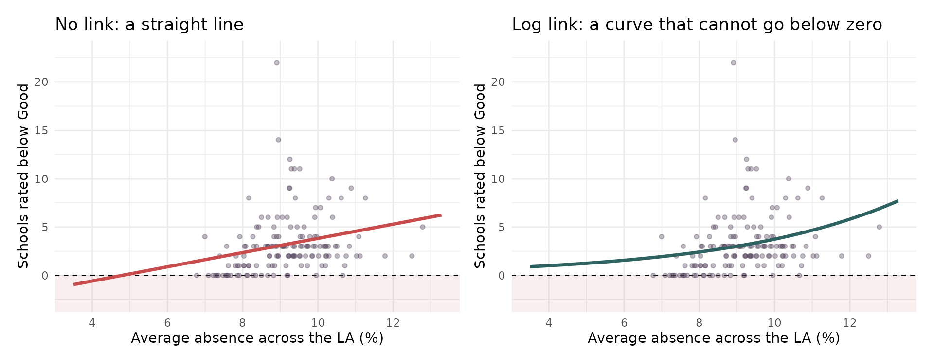
- Same data, same predictor. The straight line is heading somewhere impossible — follow it left and it promises a negative number of schools.
- The log link bends the same relationship so it flattens towards zero instead, and can never cross it.
Careful - this is not the same as logging your data
Back in Vol 1, when a relationship came out curved, we took logs of the variables and fitted OLS to the transformed numbers. That also puts a log in the model. It is not the same thing, and the difference is worth ten minutes.
What we did in Vol 1 - log(lm)
\[\log(y_i) = \beta_0 + \beta_1x_i + \epsilon_i\]
Change the data, then model it.
- Take every value of \(y\) and log it
- Fit an ordinary regression to those new numbers
- You are now modelling the average of the logged values
What a GLM does
\[\log\big(E[y_i]\big) = \beta_0 + \beta_1x_i\]
Model the data, and put the log on the model.
- Leave every value of \(y\) exactly as it is
- Work out its average, then log that
- You are modelling the log of the average
Read those two third points again. Average of the logs versus log of the average. They sound like the same sentence in a different order.
The average of the logs is not the log of the average
It comes down to which one you do first. Take three schools, with 1, 10 and 100 disadvantaged pupils.
lm - Log first, then average
(what transforming the data does)
- Log each one: 0.00, 2.30, 4.61
- Average those: 2.30
- Undo the log: 10
GLM - Average first, then log
(what a log link does)
- Add them up and divide: 37
- The model logs that: 3.61
Same three numbers. 10 against 37. Nothing has gone wrong — the order of operations simply matters, and \(\log\) is the reason why.
The same thing, on our data
The number of disadvantaged pupils across our 3,168 schools:
| What you do | Result | |
|---|---|---|
| LM - Log first, then average | log each school, average, undo the log | 38.2 pupils |
| GLM - Average first, then log | add them up and divide | 46.3 pupils |
- 8.1 pupils apart — about 17%. Not a rounding error, and not a mistake in either calculation. They are answers to different questions.
- Logging first gives you the geometric mean. Whenever a variable is skewed, it sits below the ordinary mean — and the more skewed it is, the bigger the gap.
- A model fitted to logged data is not predicting the average number of disadvantaged pupils.
- It is predicting something smaller (geometric mean), and you have to remember to say so. A log-link GLM predicts the average you actually meant.
The same gap, inside a model
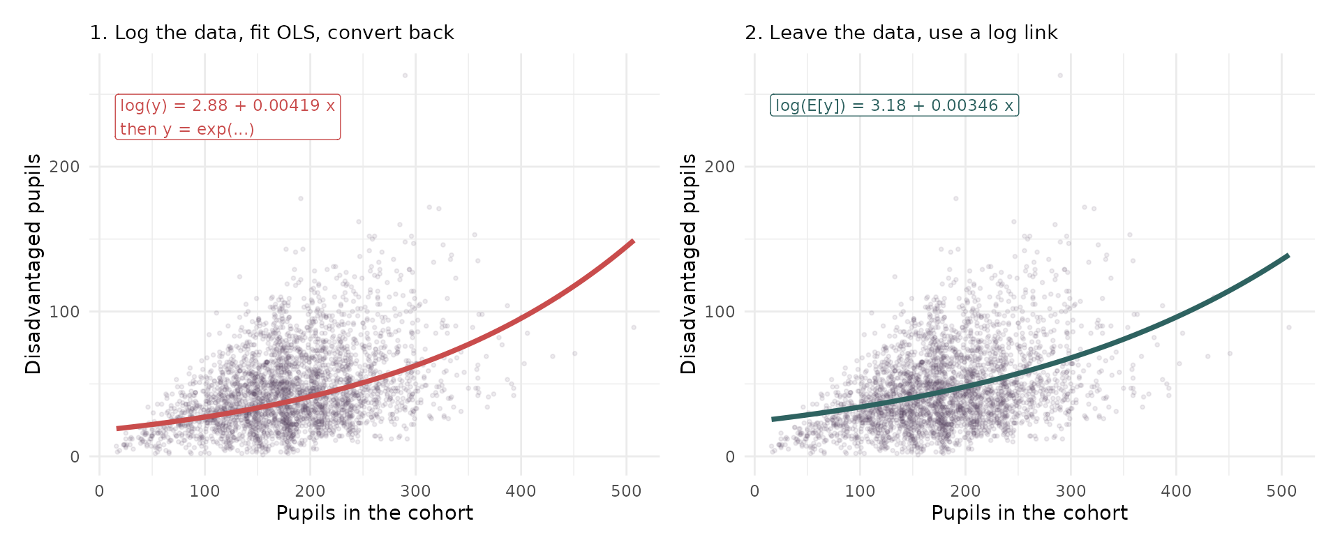
Same 3,168 schools, same predictor, both models with a log in them — and two different curves. For a cohort of 50 the left-hand route predicts about 23% fewer disadvantaged pupils than the right-hand one. The two converge as schools get bigger, which is exactly what you would expect: the more skewed the slice of data, the wider the gap.
So which one is right?
For counts, yes/no outcomes and proportions this is not a matter of taste. Logging is the wrong tool and a GLM is the right one.
For a continuous, strictly positive outcome both are defensible, and they answer slightly different questions. Four things to ask:
- What does the number have to do? If it must add up — totals, budgets, headcounts — you need the arithmetic mean, so you need the GLM. Geometric means do not aggregate. Average logged predictions across 150 LAs, convert back, and the total will be wrong
- What type is the outcome? Logging a count does not make it continuous. It makes it a logged discrete thing
- Are there zeros? Then there is no decision to make
- What do you believe about the noise? This is the real test, and it is checkable
It comes down to the errors
Logging assumes the error is multiplicative — roughly constant spread on the log scale.
A school is 20% above expectation, whatever its size.
A log-link GLM assumes the variance grows with the mean.
Bigger schools vary more in absolute terms — which is what counts actually do.
Plot the residuals against the fitted values. If the spread fans out on the raw scale but is flat once logged, logging is honest. If the variance tracks the mean, you want Poisson. This is a question you can answer with a plot, not a preference.
The published rule of thumb. O’Hara & Kotze simulated count data and compared the two approaches. Transformations performed poorly except when dispersion was small and the mean counts were large; Poisson and negative binomial models performed well throughout.
Which is exactly what the previous slide showed — 23% apart at a cohort of 50, converging to almost nothing by 400. Large counts, small gap. Small counts, big gap.
O’Hara, R.B. & Kotze, D.J. (2010) Do not log-transform count data. Methods in Ecology and Evolution, 1(2), 118–122. doi:10.1111/j.2041-210X.2010.00021.x
And sometimes you cannot transform at all
Even if you are happy with the geometric mean, transforming only works if every value can be logged. Often they cannot.
- Zeros. \(\log(0)\) is \(-\infty\). 2 of our schools have no disadvantaged pupils at all, and 24 local authorities have no below-Good schools. Every one of those rows drops out, silently
- Yes/no outcomes. A school is rated below Good or it is not. There is no scale to compress — \(\log(0)\) and \(\log(1)\) are \(-\infty\) and \(0\), and neither is any use
- The usual bodge is to log \(y + 1\) instead. It works, and it quietly changes the thing you are modelling, by an amount that depends on how big your counts are
A GLM never asks you to touch the data. The zeros stay zeros, the 0s and 1s stay 0s and 1s, and the link function does its work on the average instead — where there is nothing awkward to divide by and nothing to drop.
But hang on — what about the x variables?
In Vol 1 we did not just log the outcome. We logged the predictor too:
\[\log(y_i) = \beta_0 + \beta_1 \log(x_i) + \epsilon_i\]
A Poisson GLM looks different. The log sits on the left-hand side only:
\[\log\big(E[y_i]\big) = \beta_0 + \beta_1 x_i\]
The link is a statement about the outcome’s type. Counts cannot go negative, so we use a log link. That is all it says — and in particular it says nothing whatsoever about the predictors.
You are still free to log them, or not, exactly as you always were. That choice is untouched by the link, and we come to it next.
Logging a predictor is still available
It is just a separate decision, made for the same old reason — the relationship is curved — and completely independent of the link.
| What goes in | How you read it | |
|---|---|---|
n_below ~ mean_abs |
absence, raw | one percentage point more absence multiplies the rate by 1.25 |
n_below ~ log(mean_abs) |
absence, logged | doubling absence multiplies the rate by 4.75 |
Both are Poisson models with a log link. Both leave the outcome untouched. They differ only in whether the predictor enters raw or logged — and that changes the sentence you write, from per unit to per doubling.
Here the logged version fits slightly better (AIC 756 against 761), so it is a real choice, not a formality.
AIC is a score for comparing models fitted to the same data — lower is better. We take it apart properly later today.
One predictor we always log. Later today we add offset(log(n_schools)) to account for how many schools an LA has. That is a logged predictor with its coefficient fixed at 1 — and it is what turns a model of counts into a model of rates.
So should I log a skewed predictor?
Tempting, and a very common habit — but not because it is skewed.
Regression makes no assumption whatsoever about the distribution of your predictors. The assumptions are about the errors. A skewed x breaks nothing and is not, on its own, a problem to be fixed.
Three things that are real reasons to log a predictor:
- The relationship is curved. Straightening it is the main reason, and the only one you can see on a scatter plot
- A handful of extreme values are dragging the fit around. Logging pulls in a long tail and reduces their leverage
- You want a proportional reading — per 10% more rather than per unit more
Skew does not predict whether logging helps
| Predictor | Skew | Does logging help? |
|---|---|---|
| Pupils in the cohort | 0.37 | Yes, clearly |
| % disadvantaged | 0.79 | Yes, clearly |
| % English as an additional language | 1.59 | No - it makes it worse |
The least skewed predictor here is one where logging clearly helps. The most skewed is the one where logging actively makes the model worse.
Look at the relationship, not at the histogram of x. Skew in a predictor tells you how its values are spread out. It tells you nothing at all about whether its relationship with the outcome is straight — and that is the thing you are actually trying to fix.
So how do you tell? Draw it twice
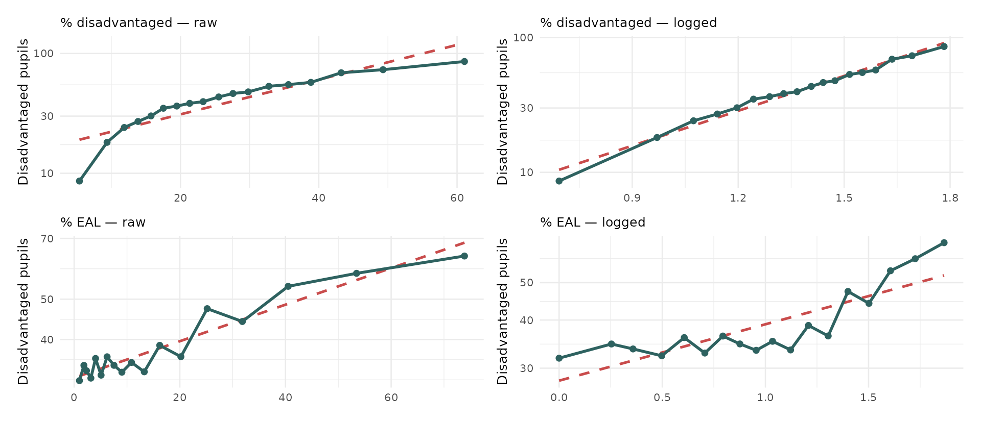
Schools split into 18 equal groups along the x-axis; each teal dot is one group’s average. Dashed is the straight line the model would fit. Where the dots wander away from the dashed line, the relationship is curved.
The tip worth remembering
Plot your outcome against the predictor twice — once raw, once logged — and keep whichever is straighter.
Put the outcome on a log axis while you do it, because that is the scale a log-link model actually works on. Straight on that plot means straight where the model cares.
On the previous slide, look at the top row: raw, the dots curve away from the line; logged, they drop neatly onto it. That is a predictor worth logging, and you can see it before fitting anything.
The bottom row does not improve. Logging the EAL figures just moves the scatter around — which is exactly why the AIC got worse when we logged it.
Three habits that will serve you all term
- Draw it before you model it — curvature is obvious in a picture and invisible in a coefficient
- Add a smoother alongside the straight line. If they agree, a straight line is fine; if they diverge, you have found something
- If logging a predictor does not visibly straighten anything, leave it alone. A transformation you cannot justify is one more thing to explain in your write-up
Can we predict School Ofsted ratings?
Our question for today
- We have used Ofsted ratings as a predictor and as a grouping variable already
- Today we turn it around and make it the outcome
- Given everything else we know about a school - its results, its intake, its absence rates, its size - can we predict what Ofsted said about it?
- And if we can, what does that tell us about what Ofsted is actually measuring?
- Note, Ofsted has changed how it rates schools now, so single-word ratings are no longer given
The outcome variable
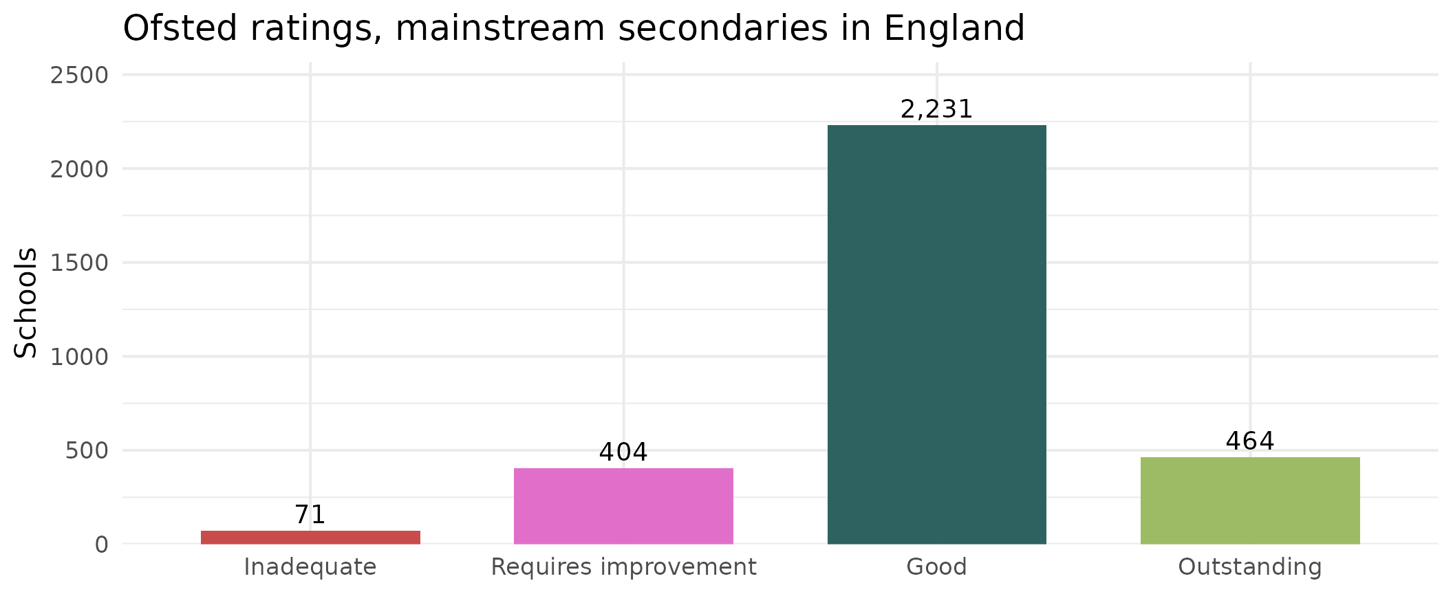
3,170 schools with complete data. Note immediately how lopsided this is - we will come back to that, because it causes more trouble than anything else today.
First attempt: just use OLS?
- Let’s re-code our ratings: “below Good” as 1 and “Good or better” as 0
- We can regress it on Progress 8 exactly as we have been doing for the last three weeks.
Call:
lm(formula = below_good ~ P8MEA, data = model_data)

Residuals:
     Min       1Q   Median       3Q      Max
-1.05109 -0.19520 -0.10193  0.03523  1.13124

Coefficients:
             Estimate Std. Error t value Pr(>|t|)
(Intercept)  0.145824   0.005812   25.09   <2e-16 ***
P8MEA       -0.274324   0.011145  -24.61   <2e-16 ***
---
Signif. codes:  0 '***' 0.001 '**' 0.01 '*' 0.05 '.' 0.1 ' ' 1

Residual standard error: 0.3271 on 3168 degrees of freedom
Multiple R-squared:  0.1606,    Adjusted R-squared:  0.1603
F-statistic: 605.9 on 1 and 3168 DF,  p-value: < 2.2e-16
The model runs. It produces coefficients. It produces an R². Nothing errors.
And its fitted values run from -0.504 to 1.051.
A probability of minus fifty percent?
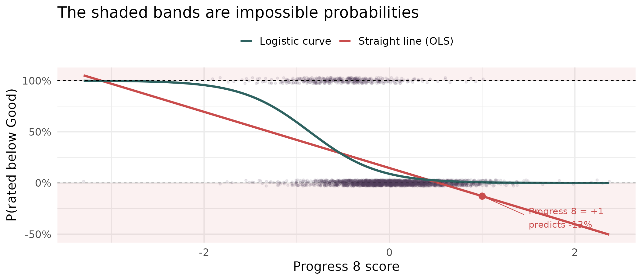
- The straight line gives 457 schools a negative probability of being rated below good.
- At a Progress 8 of +1 it predicts a probability of being rated below good of about -13% (impossible).
- The logistic curve cannot do this - it is bounded at 0 and 1 by construction.
Where the curve comes from
We need something that takes a straight line, which runs from \(-\infty\) to \(+\infty\), and squashes it into \([0,1]\).
- Start with the probability \(p\) - bounded at 0 and 1, e.g. 0.4 (40%), awkward
- Turn it into odds, \(\frac{p}{1-p} = \frac{probability of happening}{probability of NOT happening}\) or \(\frac{0.4}{0.6} = 0.67\) - now bounded at 0 and \(+\infty\), better
- Take the log of that (\(\log\left(\frac{0.4}{0.6}\right) = -0.40\)) - now unbounded in both directions 🎉
\[\log\left(\frac{p}{1-p}\right) = \beta_0 + \beta_1x_1 + \beta_2x_2 + \dots\]
- That left-hand side is the logit, and it is the link function. The right-hand side is exactly the model we have been fitting since week 5.
- A logit simply is a mathematical function that converts a probability (between 0 and 1) into a log-odds value that can range from \(-\infty\) to \(+\infty\)
- The link-function converts the expected value of the outcome (the mean) into something a straight line can cope with
Odds are not probabilities
Worth pausing, because this trips people (including me!) up all the time.
| Probability | Odds | In words |
|---|---|---|
| 0.5 | 1.0 | Evens |
| 0.75 | 3.0 | Three to one on |
| 0.9 | 9.0 | Nine to one on |
| 0.1 | 0.11 | Nine to one against |
Probabilities are bounded above. Odds are not. That is the whole reason we work with them.
And odds are not odds ratios
Odds describe one situation
\[\text{odds} = \frac{p}{1-p}\]
“This school’s odds of being rated below Good are 0.10”
An odds ratio compares two
\[\text{OR} = \frac{\text{odds}_A}{\text{odds}_B}\]
“…which is 0.07 times the odds of a school one Progress 8 point worse”
- Easily the most common mistake in reading logistic output.
- The odds are the raw ingredient;
- the ratio is what you get when you put two of them side by side - and the odds-ratio is what a regression coefficient hands you.
Why the coefficient is a ratio
First, where the “one” comes from. A slope always answers the same question, in every model you have ever fitted:
If the predictor goes up by one unit, what happens to the outcome?
In Vol 1 that was “one more percentage point of absence costs 0.38 Attainment 8 points”. The one is not special — it is just the step size we have always quoted coefficients in.
So picture two schools, identical in every respect, except the second has one more unit of \(x\) — one more percentage point of absence, say.
Why the coefficient is a ratio
Our model says the log-odds are a straight line:
\[\log(\text{odds}) = \beta_0 + \beta_1 x\]
| Predictor | Its log-odds | |
|---|---|---|
| School A | \(x\) | \(\beta_0 + \beta_1x\) |
| School B | \(x+1\) | \(\beta_0 + \beta_1x + \beta_1\) |
Subtract one from the other, and everything cancels except \(\beta_1\):
\[\log(\text{odds}_B) - \log(\text{odds}_A) = \beta_1\]
So the coefficient is a difference of two log-odds. Not a difference in probability, and not a difference in odds — a difference in logged odds.
From a difference to a ratio
We have a difference of logs. There is a rule from school algebra for exactly that:
\[\log(M) - \log(N) = \log\!\left(\frac{M}{N}\right)\]
Deliberately not A and B — those are taken. \(M\) and \(N\) are just placeholders for “whatever you are subtracting”.
Ours was \(\log(\text{odds}_B) - \log(\text{odds}_A)\), so \(M\) is School B’s odds and \(N\) is School A’s:
\[\beta_1 = \log(\text{odds}_B) - \log(\text{odds}_A) = \log\!\left(\frac{\text{odds}_B}{\text{odds}_A}\right)\]
Now undo the log on both sides — exponentiate:
\[e^{\beta_1} = \frac{\text{odds}_B}{\text{odds}_A}\]
That is the whole thing. A ratio of two odds — because subtracting logs is dividing, and the coefficient was a difference of logs all along. Nothing was smuggled in: just a one-unit step, and one rule about logarithms.
See it in our own data
That curve we drew a few slides ago had a model behind it. Here it is — the same single predictor we gave lm(), fitted properly:
(Intercept)       P8MEA
  -2.323537   -2.698673
Two numbers. That is the entire model, and it says:
\[\log(\text{odds}) = -2.32 + (-2.70 \times \text{Progress 8})\]
From those two numbers to a probability
Take a school with a Progress 8 of 0 and turn the handle. Three steps, and each one undoes a bit of the link function:
- Log-odds — put 0 into the equation: \(-2.32 + (-2.70 \times 0) = -2.32\)
- Odds — undo the log with \(\exp\): \(e^{-2.32} = 0.0979\)
- Probability — undo the odds with \(\frac{\text{odds}}{1+\text{odds}}\): \(0.0979 \div 1.0979 = 0.089\)
So a school on exactly average progress has about a 9% chance of being rated below Good.
See it in our own data
Every row below is those same three steps, done at a different Progress 8 score.
| Progress 8 | Probability | Odds | Odds ÷ the row above |
|---|---|---|---|
| -1 | 0.593 | 1.4552 | - |
| 0 | 0.089 | 0.0979 | 0.067 |
| 1 | 0.007 | 0.0066 | 0.067 |
| 2 | 0.000 | 0.0004 | 0.067 |
Check the Progress 8 = 0 row against the slide before: probability 0.089, odds 0.0979. The last column simply divides each row’s odds by the one above it.
The coefficient on Progress 8 is -2.70, and \(e^{-2.70}\) = 0.067.
That is the last column, every time. One coefficient, one odds ratio, valid wherever you start from. Now look at the probabilities - they fall 0.59 → 0.09 → 0.007, doing nothing so tidy. Which is exactly why “the probability falls by X” is never a safe reading of a logistic coefficient.
Binary logistic regression
Running the model
Same formula interface you have used for three weeks. Two differences: glm() not lm(), and a family argument.
| Term | Coefficient | Std. error | p |
|---|---|---|---|
| (Intercept) | -5.087 | 1.029 | <0.001 |
| P8MEA | -2.253 | 0.225 | <0.001 |
| PTFSM6CLA1A | -0.019 | 0.006 | 0.002 |
| PERCTOT | 0.072 | 0.080 | 0.369 |
| PPERSABS10 | 0.048 | 0.025 | 0.056 |
| log(TPUP) | 0.265 | 0.176 | 0.131 |
| PTPRIORHI | -0.006 | 0.010 | 0.571 |
| MINORGROUPMaintained school | -0.041 | 0.170 | 0.812 |
These coefficients are on the log-odds scale
- A coefficient of -2.25 on Progress 8 does not mean “the probability falls by 2.25”
- It means the log-odds fall by that much, for every one-point increase in Progress 8
- Nobody thinks in log-odds. So we exponentiate, and get an odds ratio
One extra Progress 8 point multiplies the odds of being rated below Good by about 0.11 - that is, it cuts them by roughly 89%.
Reading odds ratios
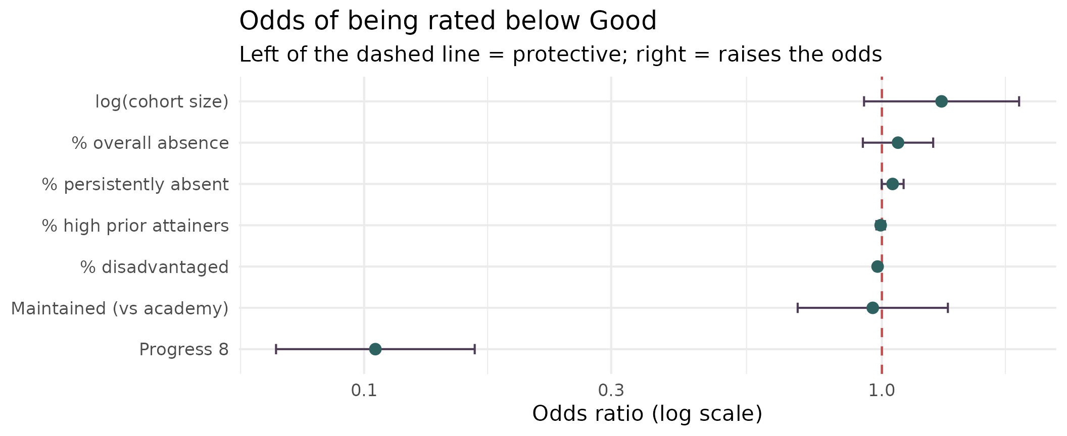
Anything whose interval crosses 1 is doing nothing detectable. Note how much work Progress 8 is doing compared with everything else.
How do you score a model like this?
For three weeks we judged models with R² — the share of the variation in the outcome the model managed to explain.
That worked because the outcome was a number, with variation in it to explain. Ours is a yes or no. There is no spread to account for, and R² as you know it simply does not exist here.
So we ask two questions instead, and they are genuinely different:
- Does the model fit the data? — likelihood, deviance, AIC, the pseudo-R²s, Hosmer–Lemeshow
- Does it make good decisions? — accuracy, the confusion matrix, ROC and AUC
A model can do respectably on one and badly on the other. We take them in turn.
1. Does the model fit?
Likelihood: how surprised is the model?
Every school in the data either was or was not rated below Good. The model assigns each one a probability. Likelihood asks the obvious question:
Given these coefficients, how probable was the data we actually saw?
- A school that was below Good, which the model gave 0.9 — good, that was likely
- A school that was not, which the model gave 0.9 — bad, the model was confidently wrong
- Multiply all 2,219 of those probabilities together and you have the likelihood of the whole dataset
Fitting the model is choosing the coefficients that make this number as large as possible — maximum likelihood. We report its log, because multiplying 2,219 probabilities together gives a number too small for a computer to hold.
For our model: log-likelihood = -717.2. Always negative; closer to zero is better.
Deviance: distance from a perfect fit
A log-likelihood on its own is hard to read. Deviance rescales it into something more like an error score — how far this model sits from one that predicted every school perfectly.
\[\text{deviance} = -2 \times \text{log-likelihood}\]
| What it is | ||
|---|---|---|
| Null deviance | 1883.4 | with no predictors at all — just the overall rate |
| Residual deviance | 1434.3 | with our seven predictors in |
Lower is better, and the drop — 449 — is what the predictors bought us. This is the direct equivalent of the sum-of-squares drop you used to read off an OLS table.
AIC: fit, minus a fine for complexity
There is a problem with judging a model on deviance alone: adding any predictor, however useless, will always lower it slightly. Left to itself, deviance always says “more variables”.
So we charge for them:
\[\text{AIC} = \text{deviance} + 2k \quad\text{where } k = \text{number of coefficients}\]
For our model: 1434.3 + 2 × 8 = 1450.3. A predictor only improves the AIC if it reduces the deviance by more than the 2 points it costs.
AIC has no meaning on its own. 1450 is neither good nor bad — it is only useful for comparing models fitted to the same data. Lower wins. That is exactly how we used it earlier to choose between a raw and a logged predictor.
The pseudo-R²s
People badly want an R², so several substitutes exist. The two you will meet in software output:
Cox & Snell — built from the likelihood ratio between your model and the null model. For us: 0.183.
That looks dismal — until you learn its catch. Cox & Snell cannot reach 1. With a binary outcome its ceiling here is 0.572, so 0.183 is really 0.183 out of a possible 0.572.
Nagelkerke fixes precisely that, by dividing by the ceiling:
\[R^2_{\text{Nagelkerke}} = \frac{0.183}{0.572} = \mathbf{0.320}\]
Now it can reach 1, and it reads much more like the R² you are used to.
…and how much to trust them
Report them if the journal or the marker expects them — but know what you are saying.
- They are not “variance explained”. Nothing here is variance. The name is borrowed, and the interpretation does not come with it
- They are not comparable across datasets, and barely across models. A Nagelkerke of 0.32 is not “half as good” as one of 0.64
- There is no accepted threshold for a good one. Values that would be embarrassing in OLS are routine here
Treat a pseudo-R² as a rough indication that the predictors are doing something, and nothing more. If you want to know whether the model is actually any use, ask the second question — the one we come to next.
Hosmer–Lemeshow: does it fit everywhere?
Everything so far gives one number for the whole model. Hosmer–Lemeshow asks something more specific: is the model well calibrated across the whole range of risk, or only in parts of it?
- Sort the schools by predicted probability and cut them into 10 equal groups
- In each group, compare how many actually were below Good with how many the model expected
- Add up the discrepancies into a chi-squared statistic
Ours: \(\chi^2\) = 11.3 on 8 df, p = 0.186.
Read the direction carefully — it is the opposite of most tests. A small p-value means the model fits badly. Ours is 0.19, so there is no evidence of poor fit.
And “no evidence of poor fit” is not the same as “good fit”. The test is known to be sensitive to how many groups you choose, and to have little power on small samples. It is a flag worth checking, not a certificate.
2. Does it make good decisions?
Don’t mark your own homework
The obvious way to answer that is to run the model over our schools and count how often it got the answer right.
The problem: it has already seen those schools. The coefficients were chosen to fit them as closely as possible. Scoring a model on the data it was fitted to is revising with the exam paper in front of you — you will do well, and it tells you nothing about the next paper.
2,219 schools to learn from, 951 kept back to test on. The model never sees the second group while it is being fitted, so how it does there is a fair sitting of a fresh paper.
That is what test-set accuracy means: of the 951 schools it had never met, what share did it classify correctly?
So how good is it?
Test-set accuracy: 86.2%
Not bad! Nearly nine schools in ten classified correctly.
Now watch.
The single most important slide today
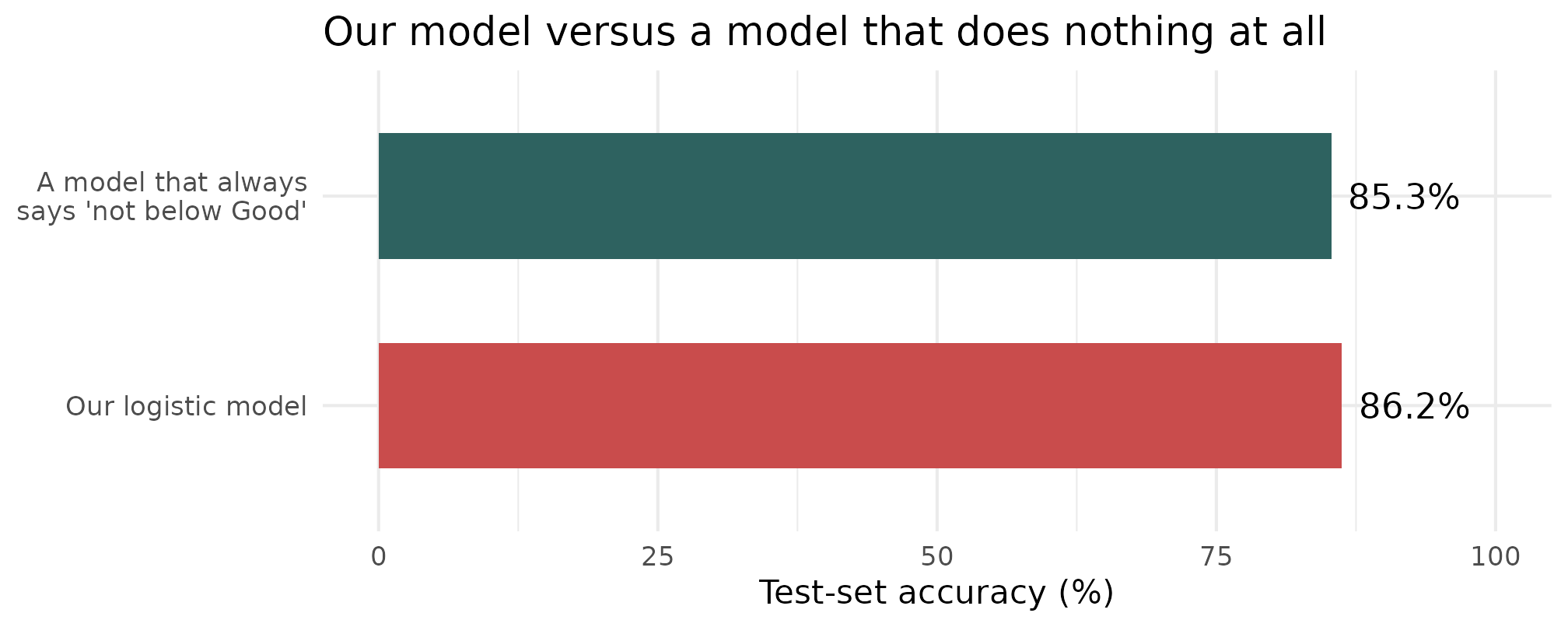
A model that makes the same prediction every single time, with no data at all, scores 85.3%. Our model beats it by 0.9 percentage points.
Why accuracy lied to us
| Predicted below Good | Predicted Good or better | |
|---|---|---|
| Actually Below Good | 32 | 108 |
| Actually Good or better | 23 | 788 |
The 951 test schools — the ones the model never saw while it was being fitted.
- Only 140 of the 951 test schools are actually below Good - the class is rare
- The model catches 32 of them and misses 108
- If you were Ofsted, trying to decide which schools to visit, this model would be close to useless at this threshold
Always, always compare your accuracy against the majority-class baseline. On imbalanced data, accuracy on its own is not evidence of anything.
0.5 was a choice, not a law
The model does not output yes or no. It outputs a probability for every school. We turned that into a yes/no by flagging anything above 0.5 — and nothing made 0.5 the right number.
| Flag if probability above | Struggling schools caught | …and missed | False alarms |
|---|---|---|---|
| 0.50 | 32 | 108 | 23 |
| 0.30 | 57 | 83 | 75 |
| 0.20 | 91 | 49 | 134 |
| 0.10 | 121 | 19 | 316 |
Drop the threshold and you catch far more struggling schools — 32 up to 121 of the 140. But the false alarms go from 23 to 316.
There is no setting that is simply best. Which error hurts more is a policy question, and the model cannot answer it for you.
Every threshold at once: the ROC curve
Rather than argue about one cut-off, plot all of them. Two numbers per threshold:
- True positive rate — of the schools that really are below Good, what share did we flag? (we want this high)
- False positive rate — of the schools that are fine, what share did we flag anyway? (we want this low)
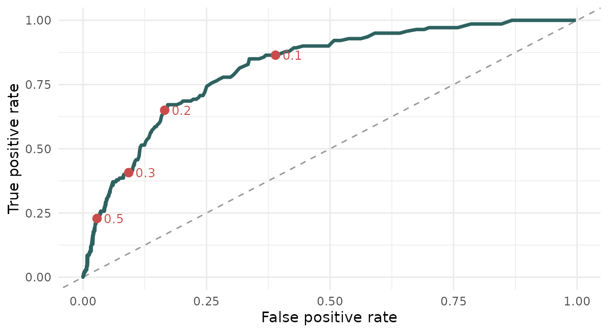
Each red dot is one row of the table above. Sweep the threshold from 1 down to 0 and you trace the whole curve. The dashed diagonal is what you would get by guessing at random — the further above it you sit, the more the model knows.
And AUC is the area underneath it
One curve is awkward to quote in a sentence, so we summarise it by the area under it — the AUC.
| AUC | What it means |
|---|---|
| 0.5 | the diagonal — no better than tossing a coin |
| 0.7–0.8 | useful |
| 0.9+ | very strong |
| 1.0 | perfect: every struggling school scored above every healthy one |
It also has a reading that needs no curve at all:
Pick one struggling school and one healthy school at random. AUC is the probability the model gives the struggling one the higher score.
Notice what that does not depend on: any threshold. AUC asks whether the model puts schools in the right order, which is a different and fairer question from whether it labels them correctly at one arbitrary cut-off.
But the model is not useless
Accuracy asks “did you get it right?” at one arbitrary cut-off. A better question is “do you rank schools sensibly?”
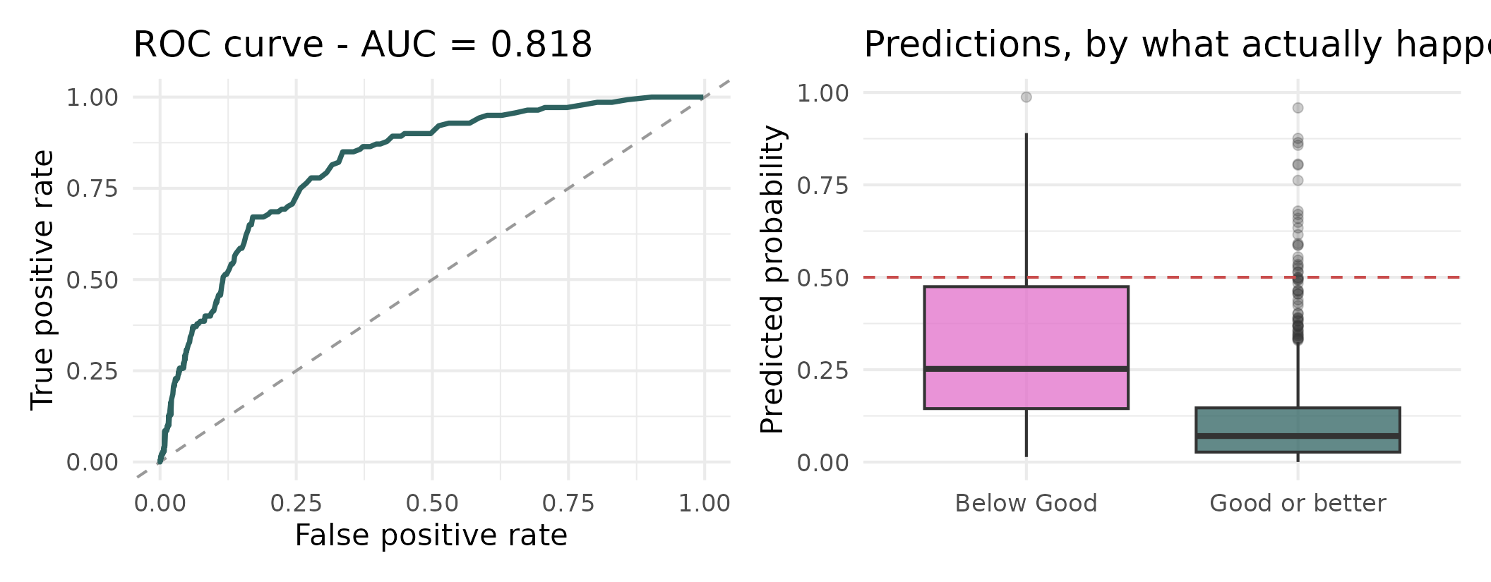
AUC = 0.818 - pick a below-Good school and a Good-or-better school at random, and the model gives the below-Good one a higher score 82% of the time. That is genuinely useful. The problem was never the model - it was the 0.5 threshold, which is a choice, not a law.
Moving the threshold
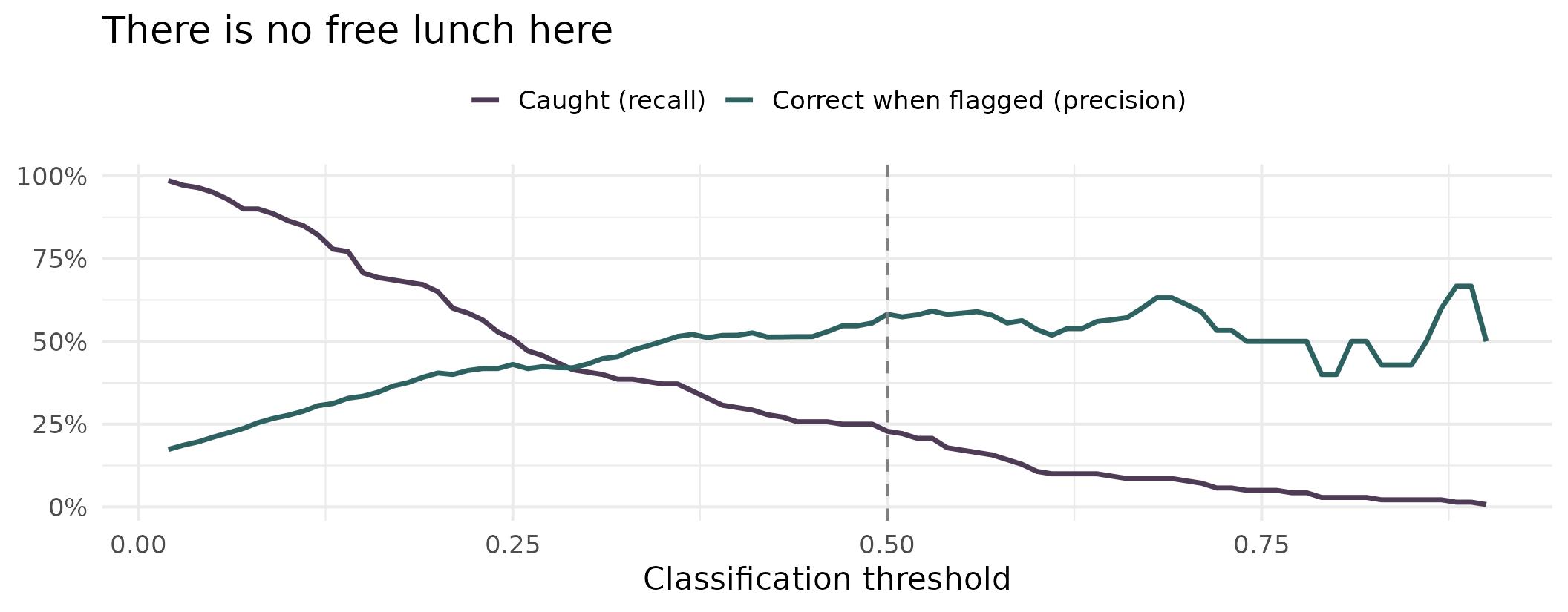
Drop the threshold and you catch more struggling schools, but more of your flags are false alarms. Which error is worse is a policy question, not a statistical one - and that is the right way round.
A second outcome, same story
| Model | Accuracy | Baseline | AUC | Caught at p > 0.5 |
|---|---|---|---|---|
| Below Good vs Good+ | 86.2% | 85.3% | 0.818 | 32 of 140 |
| Outstanding vs rest | 88.3% | 85.6% | 0.896 | 52 of 137 |
- Higher AUC, so the ranking is even better
- Barely above baseline on accuracy, and still catching well under half the Outstanding schools
- Not a quirk of one model. This is what rare outcomes do, and you will meet it in your own data
An uncomfortable question
Progress 8 is by far the strongest predictor in both models. So what have we actually built?
- Ofsted inspectors read a school’s Progress 8 score before they visit
- So we are not independently predicting a judgement - we are partly recovering one of Ofsted’s own inputs
- That is circularity, and it makes the model much less interesting than it first looked
And a second problem: inspection dates in this file run from 2011 to 2024, median 2022. Some of these ratings were handed out a decade before the results we are using to “predict” them.
Ask these questions of your own models. They matter more than another decimal place of AUC.
Categories with an order
We threw information away
- To fit a binary model, we collapsed four ratings into two
- But Ofsted ratings have an obvious order: Inadequate < Requires improvement < Good < Outstanding
- Treating them as a number (1, 2, 3, 4) is the mistake we warned about in week 1 - it assumes the gaps are equal
- Treating them as unordered throws away real information
Ordinal logistic regression uses the order without assuming the spacing.
The idea: cut points on a hidden scale
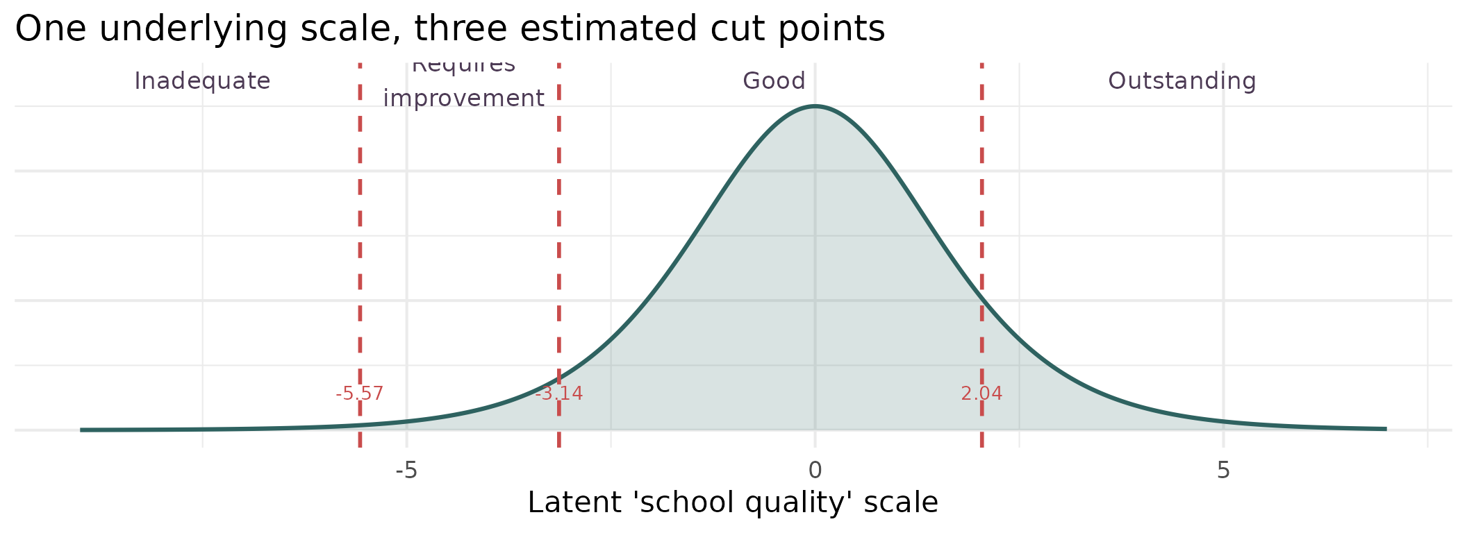
We imagine a single continuous scale we cannot observe. The predictors move a school along it, and the cut points decide which rating it comes out as. Three cut points for four categories - and the model estimates them from the data rather than assuming them.
Running it
| Term | Value | t | p |
|---|---|---|---|
| P8MEA | 2.748 | 16.85 | <0.001 |
| PTFSM6CLA1A | 0.019 | 4.24 | <0.001 |
| PERCTOT | -0.048 | -0.74 | 0.459 |
| PPERSABS10 | -0.041 | -2.18 | 0.029 |
| log(TPUP) | 0.045 | 0.35 | 0.73 |
| PTPRIORHI | 0.013 | 3.44 | <0.001 |
| MINORGROUPMaintained school | -0.131 | -1.04 | 0.3 |
| Inadequate|Requires improvement | -5.572 | -7.11 | <0.001 |
| Requires improvement|Good | -3.136 | -4.10 | <0.001 |
| Good|Outstanding | 2.042 | 2.67 | 0.008 |
The last three rows are the cut points, not predictors. Everything above them reads like a logistic model: positive means more likely to be rated higher.
Did it work?
| Inadequate | Requires improvement | Good | Outstanding | |
|---|---|---|---|---|
| Inadequate | 0 | 5 | 13 | 0 |
| Requires improvement | 3 | 21 | 98 | 0 |
| Good | 2 | 25 | 628 | 19 |
| Outstanding | 0 | 0 | 92 | 45 |
- Accuracy 73.0% against a baseline of 70.9%
- It never once correctly predicts Inadequate - 0 out of 18
- But it is within one category 98.4% of the time
So: can we predict Ofsted?
Roughly, yes. Precisely, no. And the rare categories, not at all.
- The model knows the difference between a likely-Outstanding school and a likely-struggling one
- It cannot tell you which side of a single grade boundary a school will land
- And it has essentially never seen enough Inadequate schools to learn what they look like
That is an honest, useful answer - and a far better one than a single accuracy figure would have given you.
Categories without an order
When there is no natural ordering
- Ofsted ratings are ordered, so ordinal logistic is the right tool
- But plenty of categorical outcomes are not: which region a school is in, which type of school a pupil moves to, which of five clusters a neighbourhood falls into
- Multinomial logistic regression handles those - it fits a separate set of coefficients for every category against a reference
Let’s fit it to Ofsted anyway, deliberately ignoring the order, to see what ignoring the order costs us.
The comparison
| Model | Parameters | Test accuracy | AIC |
|---|---|---|---|
| Ordinal (proportional odds) | 10 | 73.0% | 2921 |
| Multinomial | 24 | 73.7% | 2877 |
- The multinomial buys about 0.7 of a percentage point of accuracy
- It spends more than twice as many parameters to get it
- AIC mildly prefers it, which tells us the proportional-odds assumption is not perfectly met
Use the structure in your data when you have it. The ordinal model gets almost the same performance from a third of the coefficients, and you can actually interpret it.
Counting things
A different kind of outcome
Let’s change the question and move up a level.
How many below-Good schools does each local authority have?
- That is a count: 0, 1, 2, 3… never negative, never fractional
- Most LAs have a few; some have none at all; a couple have a lot
- A straight line will happily predict minus two struggling schools, which is not a thing
What counts look like
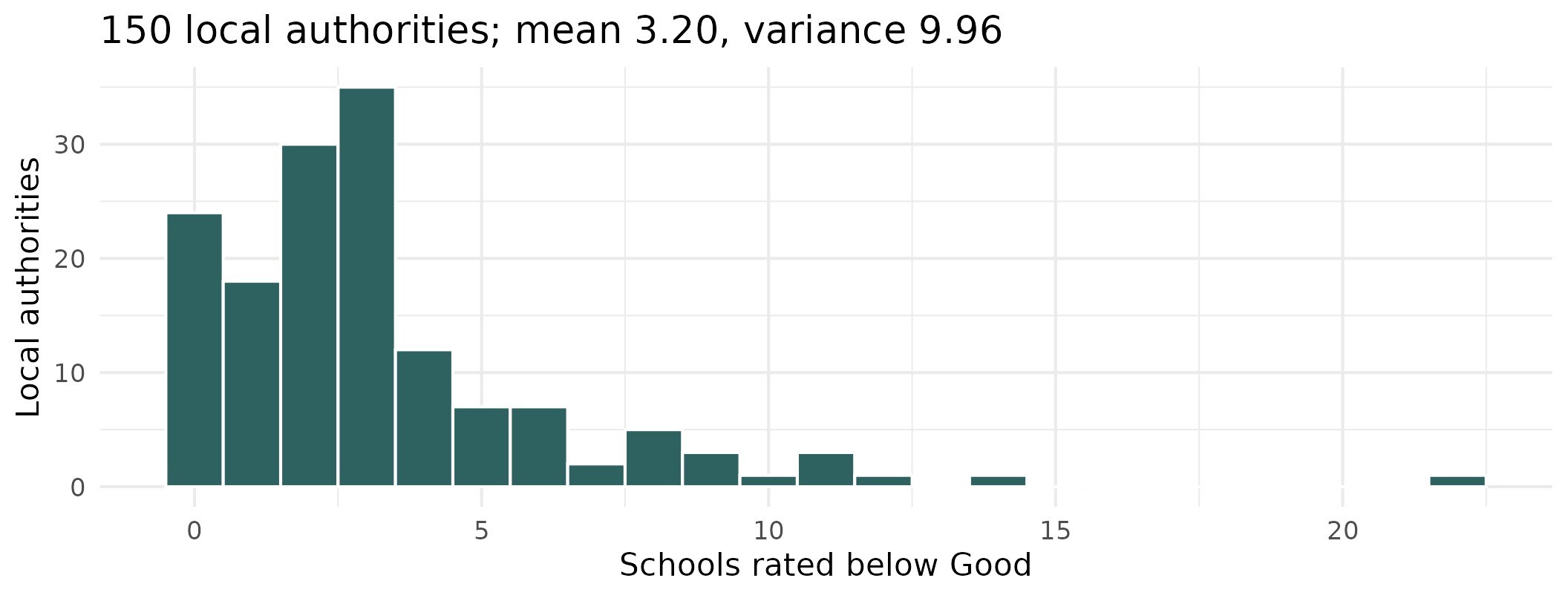
Discrete, non-negative, right-skewed, with a pile-up at the low end - 24 LAs have no below-Good schools at all. This is a Poisson-shaped problem, exactly as week 1 described.
But first - counts or rates?
| Local authority | Secondary schools | Rated below Good | As a share |
|---|---|---|---|
| Lancashire | 78 | 22 | 28% |
| Bury | 13 | 6 | 46% |
On the raw count, Lancashire looks nearly four times worse. On the share, Bury is the one in trouble.
A count on its own tells you very little, because it depends on how many chances there were to begin with. Lancashire has six times as many schools, so it would take more below-Good ones even if nothing were wrong.
So why not just divide?
The obvious move is to model the share — n_below / n_schools — and be done with it. Two reasons not to:
- Poisson describes whole numbers.
22/79 = 0.28is not a count of anything. We would be using a distribution for something it does not describe - Dividing throws away how much evidence you have. Bury’s 46% rests on 13 schools. Lancashire’s 28% rests on 79. We should be far more confident about Lancashire — but once both are just “a percentage”, the model can no longer tell them apart
An offset gets us both: the outcome stays a genuine count, so Poisson still applies and the sample sizes still count for something — but the model does the dividing internally.
What an offset actually is
Three lines of algebra, and nothing clever happens in any of them.
1. What we actually want to model — a rate, not a count:
\[\log\left(\frac{\text{expected count}}{\text{number of schools}}\right) = \beta_0 + \beta_1x\]
2. The log of a ratio is a difference of logs — ordinary school algebra:
\[\log(\text{expected count}) - \log(\text{number of schools}) = \beta_0 + \beta_1x\]
3. Move that term across to the other side:
\[\log(\text{expected count}) = \beta_0 + \beta_1x + \log(\text{number of schools})\]
That final term — \(\log(\text{number of schools})\) — is the offset.
So an offset is just a division, rewritten as an addition so it can sit inside a model that works on the log scale. In R that is offset(log(n_schools)).
Fixed, not estimated
Look at line 3 again. Every other term on the right gets a \(\beta\) in front of it that the model chooses. The offset does not — it is stuck there with a coefficient of exactly 1, because that is how it arrived.
In plain words, we are telling the model something rather than asking it:
Twice as many schools, twice as many below-Good ones expected, all else being equal.
That is a claim about arithmetic, not about education policy, so we spend no parameter finding it out.
Is that a fair thing to assume? Put log(n_schools) in as an ordinary predictor and let the model estimate it instead. It comes back with 0.95, with a 95% interval of 0.82 to 1.09 — 1 sits comfortably inside it. The assumption holds, and fixing it saves us a parameter.
Always worth checking. If that interval had excluded 1, the offset would have been the wrong tool.
Running a Poisson model
| Term | Coefficient | Rate ratio | p |
|---|---|---|---|
| (Intercept) | -4.4903 | 0.011 | <0.001 |
| Mean % disadvantaged | -0.0017 | 0.998 | 0.751 |
| Mean % absence | 0.2834 | 1.328 | <0.001 |
The link function here is \(\log\), so exponentiating gives a rate ratio. And note the result: once average absence is in the model, average disadvantage adds nothing detectable - a confounding story of exactly the kind we met in week 6.
Checking the Poisson assumption
The Poisson distribution assumes something quite strong: that the variance equals the mean. Real data often disagrees.
A value near 1 means the assumption holds. Much above 1 means overdispersion - the data are more variable than Poisson allows, your standard errors are too small, and you will think results are significant when they are not.
Here we get 1.31, which is mild. So Poisson is adequate - but we should check rather than assume.
When it is not adequate
| Model | AIC | SE on absence |
|---|---|---|
| Poisson | 577 | 0.0485 |
| Negative binomial | 575 | 0.0528 |
- The negative binomial is the Poisson’s more forgiving cousin - it adds a parameter that lets the variance exceed the mean
- This is exactly the distribution we met in week 1, and this is what it is for
- Here the two models are essentially tied, so we keep the simpler one
Fit the Poisson, check the dispersion, escalate only if you need to.
The fun bit: who beats their own odds?
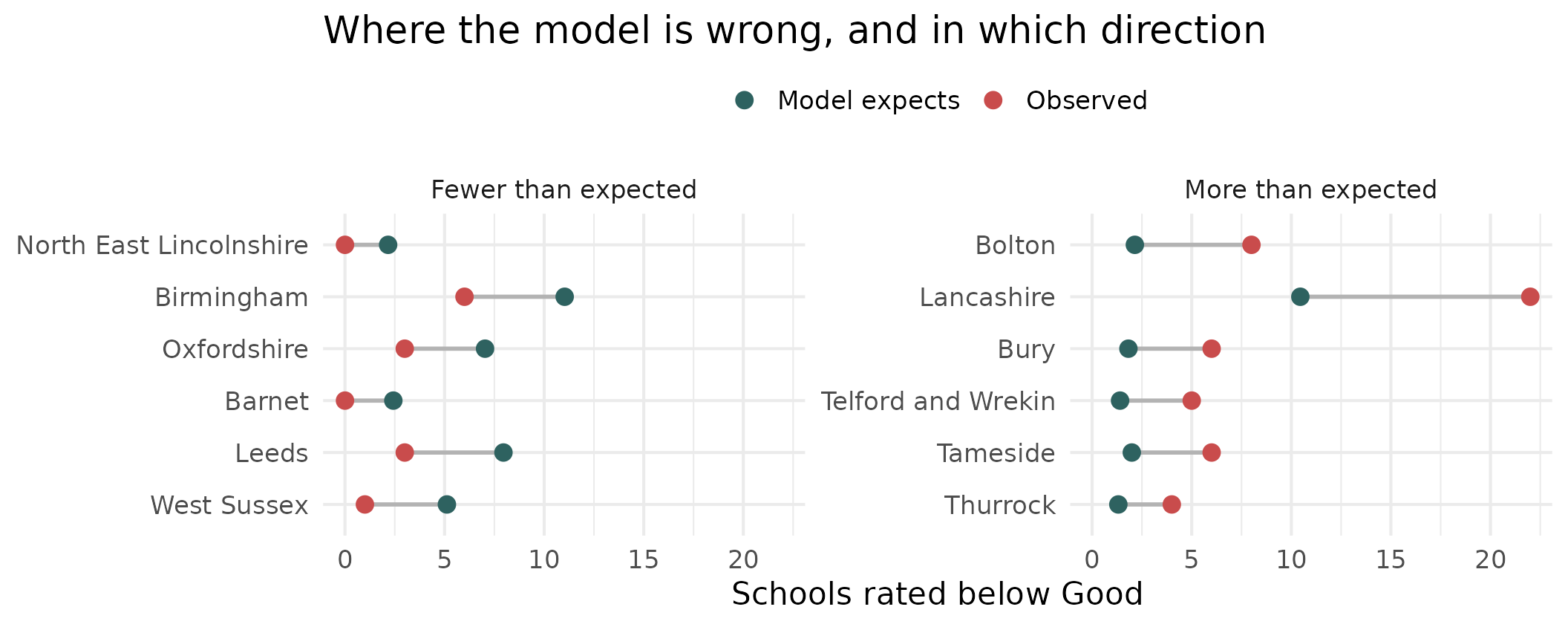
Given their intake, some LAs have far more struggling schools than expected and some far fewer. The residuals of a count model are not a diagnostic afterthought here - they are the finding.
One more outcome type
Proportions out of a known total
Back down to school level, and to a file we have not touched yet: what happens to pupils after Year 11?
| Value | |
|---|---|
| Schools | 3,081 |
| Median cohort | 175 |
| Median % sustaining a destination | 94.4% |
| Schools at exactly 100% | 48 (1.6%) |
- Each school gives us “x of n pupils went on to education, employment or training”
- That is not really a percentage - it is a count out of a known total, which is exactly what the binomial distribution describes
Modelling it properly
Note the cbind() - we hand the model successes and failures, not a proportion, so it knows a school of 30 carries less weight than a school of 300.
Every 10 percentage points more disadvantage is associated with a 23% fall in the odds of a pupil sustaining a destination.
Does it matter? Compare the predictions
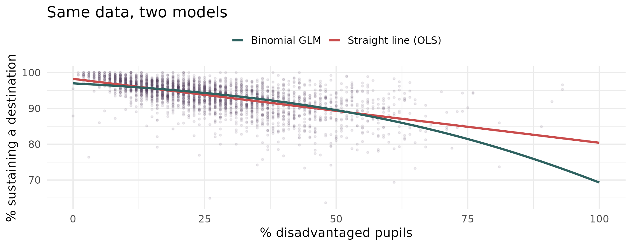
They agree almost exactly through the middle and diverge at the top end - the schools policy cares about most. Here OLS is not obviously broken. It is quietly wrong at the edges, and nothing in its output tells you so.
And check the dispersion again
| Model | Dispersion | Verdict |
|---|---|---|
| LA below-Good counts (Poisson) | 1.31 | Mild - Poisson is fine |
| Destinations (binomial) | 2.72 | Overdispersed - use quasibinomial |
- Two models, two different answers. The check is not a formality you tick off
- For the destinations model, switching to
family = quasibinomialwidens the standard errors by about 60% - the coefficients are unchanged, but our confidence in them was overstated
Wrapping up
The family, in one slide
| Outcome | family = |
Link | Interpret coefficients as |
|---|---|---|---|
| Continuous | gaussian |
identity | Units of y per unit of x |
| Yes / no | binomial |
logit | Odds ratios |
| x out of n | binomial |
logit | Odds ratios |
| Ordered categories | MASS::polr() |
logit | Odds of being in a higher category |
| Unordered categories | nnet::multinom() |
logit | Odds vs a reference category |
| Count | poisson |
log | Rate ratios |
| Overdispersed count | MASS::glm.nb() |
log | Rate ratios |
One framework. Change the family, change the link, and everything you learned about building and interpreting a linear model still applies.
What carried over, and what didn’t
Still true
- The recipe: start simple, add complexity that earns its place
- Confounding, mediation, interactions
- Multicollinearity and VIF
- Thinking hard about what belongs in the model
Different now
- No R² - use AIC, deviance, or predictive performance
- Coefficients need exponentiating before they mean anything
- Residual plots look strange and need different diagnostics
- Accuracy is a trap on imbalanced outcomes
Where you can go next
- Generalised additive models (GAMs) - when the relationship is smooth but not a straight line
glmer()- the intersection of this week and last week: a GLM with random effects, for grouped non-normal data- Spatial and geographically weighted regression - when the relationship itself varies over space
- Ridge and lasso - when you have too many predictors and need the model to choose
You now have the two big extensions to OLS: last week we relaxed independence, this week we relaxed normality. Almost everything else is a combination of the two.
Conclusions
- Look at your outcome variable before you choose a model. Week 1’s data types were not an academic exercise - they determine what you are allowed to do
- A GLM is not a new method, it is the same linear predictor with a different distribution and a link function bolted on
- Always compare against a baseline. A model that beats “predict the majority every time” by half a percentage point has not learned much
- Check your assumptions - dispersion for counts, and the threshold question for classification
- And ask where your predictors came from. Our best one turned out to be something Ofsted had already read
Today’s Practical
- Building and interpreting your own logistic and Poisson models on the schools data
- Practice at the bit that matters most: interpreting odds ratios and rate ratios in plain English
- And deciding, for an outcome of your own choosing, which member of the family you actually need

© CASA | ucl.ac.uk/bartlett/casa