Prof D’s Regression Sessions - Vol 5
Counts, rates and the negative binomial
Adam Dennett - a.dennett@ucl.ac.uk
Week GLM
CASA0007 Quantitative Methods
Last time
- We met the Generalised Linear Model — one framework, three moving parts: a distribution, a linear predictor, and a link function
- We spent the session on logistic regression, because once you can read an odds ratio the rest of the family follows
- And we left three outcome types on the table. This session picks up the biggest of them: counts
This session
- \(E[y]\) — the notation the count models are written in, and why it is nothing new
- Poisson regression for counts, and how to read a rate ratio
- Offsets — the thing that turns a model of counts into a model of rates, which is almost always what you actually wanted
- Overdispersion, and the negative binomial model that deals with it
- Proportions — x out of n — which turn out to be a binomial problem in disguise
Same dataset, same schools. The only thing changing is what we put on the left-hand side.
First, a word on notation
A quick word on \(E[y]\)
With GLMs there is an \(E\) in most of the equations. \(E\) is for expectation, and \(E[y_i]\) reads “the expected value of y for school i”.
- It is essentially an average — but a theoretical one. Your sample mean is a fact about the 3,000 schools you happen to have; an expected value is a fact about the process that produced them
- “Expected” is a poor name. It need not be a value you could ever observe — the expected value of a dice roll is 3.5, and the expected number of children per family is about 1.8
- The little \(i\) matters. \(E[y_i]\) is that school’s own expected value, and it depends on that school’s predictors. There are thousands of them, one per school — not a single average across the dataset
You have been using it all along
Ordinary regression, exactly as we wrote it in Vol 1:
\[y_i = \beta_0 + \beta_1x_i + \epsilon_i\]
The errors average out to zero. So take the average of both sides, and the error term disappears:
\[E[y_i] = \beta_0 + \beta_1x_i\]
That is the line you have been drawing through scatter plots since week 5. - A regression line was never an exact school prediction — It is a prediction of what the average school like it does - this is the expected value
So \(\log(E[y_i])\) is not anything new or different. Just more formalised in the GLM equation.
The same model, three times
Written out in full, with the right-hand side identical every time. Only the left changes.
Ordinary regression — the outcome goes in as it is:
\[y_i = \beta_0 + \beta_1x_1 + \beta_2x_2 + \dots + \epsilon_i\]
Logistic regression — last session. The probability goes in, through the logit:
\[\log\!\left(\frac{p_i}{1-p_i}\right) = \beta_0 + \beta_1x_1 + \beta_2x_2 + \dots\]
Poisson regression — today. The expected count goes in, through a log:
\[\log\big(E[y_i]\big) = \beta_0 + \beta_1x_1 + \beta_2x_2 + \dots\]
Notice what is missing from the bottom two: the \(\epsilon\). OLS adds an error term on the end; a GLM does not, because the randomness is already described by the distribution you chose. That is the swap — an error term for a distribution.
Counting things
A different kind of outcome
Let’s change the question and move up a level.
How many below-Good schools does each local authority have?
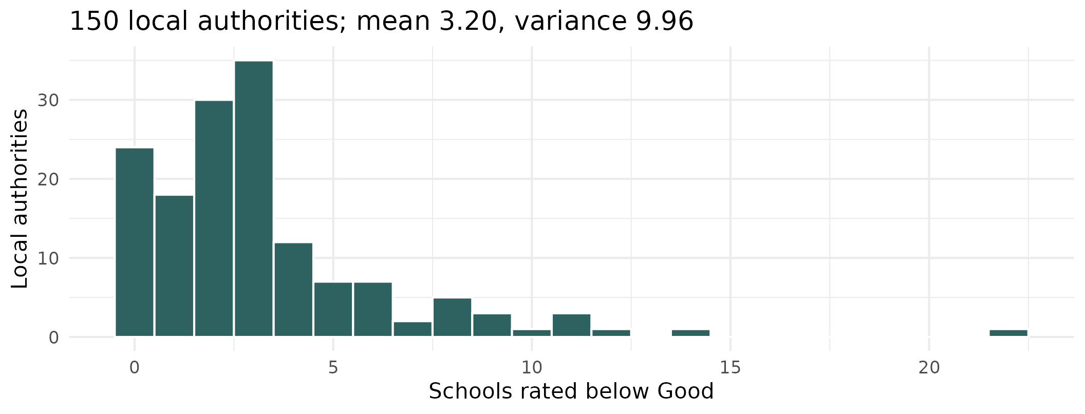
- That is a count: 0, 1, 2, 3… never negative, never fractional
- Most LAs have a few; some have none at all; a couple have a lot
- A straight line will happily predict minus two struggling schools, which is not a thing
What counts look like
Discrete, non-negative, right-skewed, with a pile-up at the low end - 24 LAs have no below-Good schools at all. This is a Poisson-shaped problem, exactly as week 1 described.
But first - counts or rates?
| Local authority | Secondary schools | Rated below Good | As a share |
|---|---|---|---|
| Lancashire | 78 | 22 | 28% |
| Bury | 13 | 6 | 46% |
On the raw count, Lancashire looks nearly four times worse. On the share, Bury is the one in trouble.
A count on its own tells you very little, because it depends on how many chances there were to begin with. Lancashire has six times as many schools, so it would take more below-Good ones even if nothing were wrong.
So why not just divide?
The obvious move is to model the share — n_below / n_schools — and be done with it. Two reasons not to:
- Poisson describes whole numbers.
22/79 = 0.28is not a count of anything. We would be using a distribution for something it does not describe - Dividing throws away how much evidence you have. Bury’s 46% rests on 13 schools. Lancashire’s 28% rests on 79. We should be far more confident about Lancashire — but once both are just “a percentage”, the model can no longer tell them apart
An offset gets us both: the outcome stays a genuine count, so Poisson still applies and the sample sizes still count for something — but the model does the dividing internally.
What an offset actually is
Three lines of algebra, and nothing clever happens in any of them.
1. What we actually want to model — a rate, not a count:
\[\log\left(\frac{\text{expected count}}{\text{number of schools}}\right) = \beta_0 + \beta_1x\]
2. The log of a ratio is a difference of logs — ordinary school algebra:
\[\log(\text{expected count}) - \log(\text{number of schools}) = \beta_0 + \beta_1x\]
3. Move that term across to the other side:
\[\log(\text{expected count}) = \beta_0 + \beta_1x + \log(\text{number of schools})\]
That final term — \(\log(\text{number of schools})\) — is the offset.
So an offset is just a division, rewritten as an addition so it can sit inside a model that works on the log scale. In R that is offset(log(n_schools)).
Fixed, not estimated
Look at line 3 again. Every other term on the right gets a \(\beta\) in front of it that the model chooses. The offset does not — it is stuck there with a coefficient of exactly 1, because that is how it arrived.
In plain words, we are telling the model something rather than asking it:
Twice as many schools, twice as many below-Good ones expected, all else being equal.
That is a claim about arithmetic, not about education policy, so we spend no parameter finding it out.
Is that a fair thing to assume? Put log(n_schools) in as an ordinary predictor and let the model estimate it instead. It comes back with 0.95, with a 95% interval of 0.82 to 1.09 — 1 sits comfortably inside it. The assumption holds, and fixing it saves us a parameter.
Always worth checking. If that interval had excluded 1, the offset would have been the wrong tool.
Running a Poisson model
| Term | Coefficient | Rate ratio | p |
|---|---|---|---|
| (Intercept) | -4.4903 | 0.011 | <0.001 |
| Mean % disadvantaged | -0.0017 | 0.998 | 0.751 |
| Mean % absence | 0.2834 | 1.328 | <0.001 |
The link function here is \(\log\), so exponentiating gives a rate ratio. And note the result: once average absence is in the model, average disadvantage adds nothing detectable - a confounding story of exactly the kind we met in week 6.
Checking the Poisson assumption
The Poisson distribution assumes something quite strong: that the variance equals the mean. Real data often disagrees.
A value near 1 means the assumption holds. Much above 1 means overdispersion - the data are more variable than Poisson allows, your standard errors are too small, and you will think results are significant when they are not.
Here we get 1.31, which is mild. So Poisson is adequate - but we should check rather than assume.
When it is not adequate
| Model | AIC | SE on absence |
|---|---|---|
| Poisson | 577 | 0.0485 |
| Negative binomial | 575 | 0.0528 |
- The negative binomial is the Poisson’s more forgiving cousin - it adds a parameter that lets the variance exceed the mean
- This is exactly the distribution we met in week 1, and this is what it is for
- Here the two models are essentially tied, so we keep the simpler one
Fit the Poisson, check the dispersion, escalate only if you need to.
The fun bit: who beats their own odds?
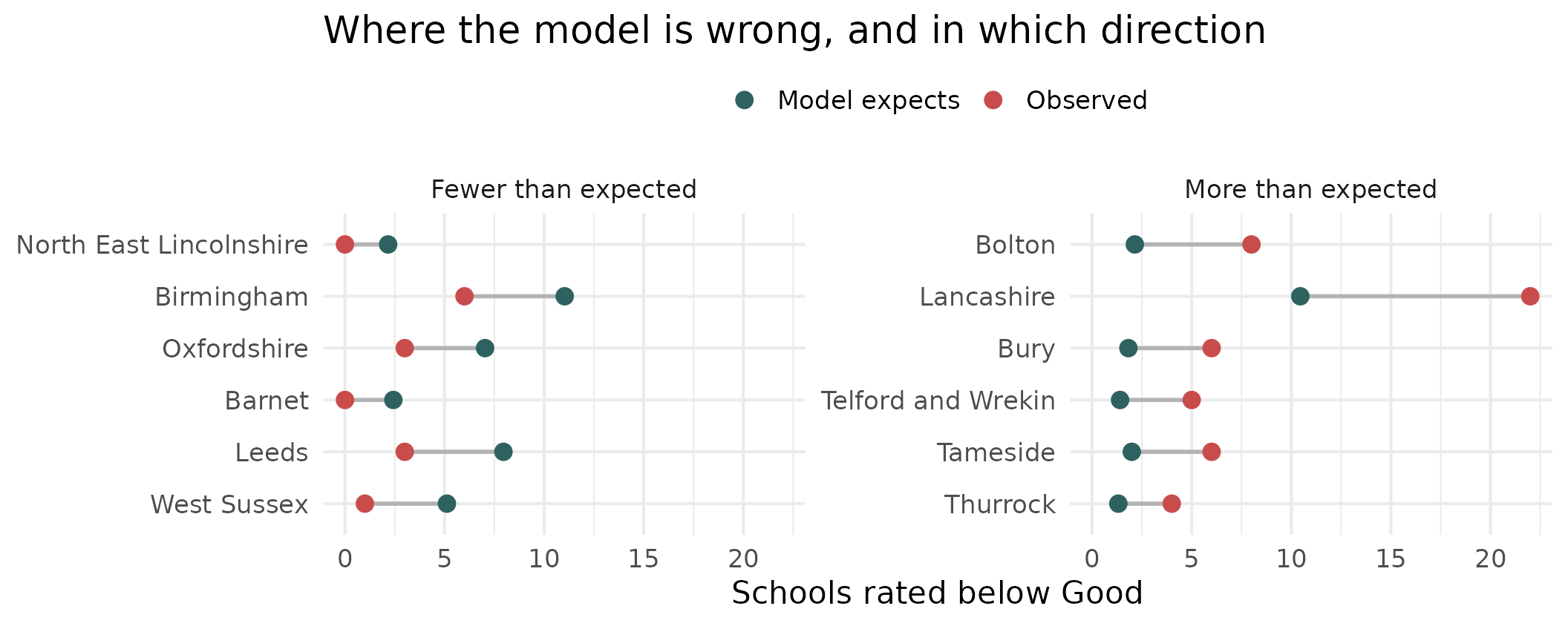
Given their intake, some LAs have far more struggling schools than expected and some far fewer. The residuals of a count model are not a diagnostic afterthought here - they are the finding.
One more outcome type
Proportions out of a known total
Back down to school level, and to a file we have not touched yet: what happens to pupils after Year 11?
| Value | |
|---|---|
| Schools | 3,081 |
| Median cohort | 175 |
| Median % sustaining a destination | 94.4% |
| Schools at exactly 100% | 48 (1.6%) |
- Each school gives us “x of n pupils went on to education, employment or training”
- That is not really a percentage - it is a count out of a known total, which is exactly what the binomial distribution describes
Modelling it properly
Note the cbind() - we hand the model successes and failures, not a proportion, so it knows a school of 30 carries less weight than a school of 300.
Every 10 percentage points more disadvantage is associated with a 23% fall in the odds of a pupil sustaining a destination.
Does it matter? Compare the predictions
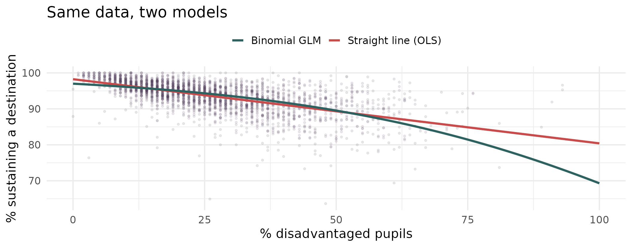
They agree almost exactly through the middle and diverge at the top end - the schools policy cares about most. Here OLS is not obviously broken. It is quietly wrong at the edges, and nothing in its output tells you so.
And check the dispersion again
| Model | Dispersion | Verdict |
|---|---|---|
| LA below-Good counts (Poisson) | 1.31 | Mild - Poisson is fine |
| Destinations (binomial) | 2.72 | Overdispersed - use quasibinomial |
- Two models, two different answers. The check is not a formality you tick off
- For the destinations model, switching to
family = quasibinomialwidens the standard errors by about 60% - the coefficients are unchanged, but our confidence in them was overstated
Wrapping up
The family, in one slide
| Outcome | family = |
Link | Interpret coefficients as |
|---|---|---|---|
| Continuous | gaussian |
identity | Units of y per unit of x |
| Yes / no | binomial |
logit | Odds ratios |
| x out of n | binomial |
logit | Odds ratios |
| Ordered categories | MASS::polr() |
logit | Odds of being in a higher category |
| Unordered categories | nnet::multinom() |
logit | Odds vs a reference category |
| Count | poisson |
log | Rate ratios |
| Overdispersed count | MASS::glm.nb() |
log | Rate ratios |
One framework. Change the family, change the link, and everything you learned about building and interpreting a linear model still applies.
Conclusions
- A count is not a continuous number. It cannot go negative, it comes in whole units, and its variance grows with its mean — so it gets a log link and a Poisson distribution
- An offset is a division in disguise. It turns counts into rates, and it is the single most commonly forgotten piece of a count model
- Always check the dispersion. Much above 1 and your standard errors are too small, which means significance you have not earned
- A proportion out of a known total is a binomial, not a percentage to be modelled with OLS —
cbind(successes, failures)keeps the sample sizes in the model where they belong
And the thread running through both sessions: look at your outcome variable before you choose a model. Week 1’s data types were never an academic exercise — they decide what you are allowed to do.
Today’s Practical
- Fitting Poisson models to the schools data, with and without an offset, and seeing what the offset changes
- Checking dispersion, and deciding whether you need the negative binomial
- Reading rate ratios out loud in plain English — the same skill as odds ratios, one family along

© CASA | ucl.ac.uk/bartlett/casa