Exploratory Data Analysis #1

Part 1 - describing what you have

Adam Dennett - a.dennett@ucl.ac.uk

18 September 2026

CASA0007 Quantitative Methods

This week

Understanding and describing data

• Quantitative methods describe the range of mathematical and statistical techniques we can apply to data in order that we can derive meaning from it
• Data may arrive in many different forms
  • spreadsheets of numbers
  • pages of text
  • ridges on a vinyl record
• Being able to identify the type of data you are dealing with will allow you to select the appropriate methods for making sense of it.

This lecture focuses on understanding and describing data.

Everything this week uses the dataset we will keep coming back to all term, so that by week 10 it is completely familiar.

Survey before you build

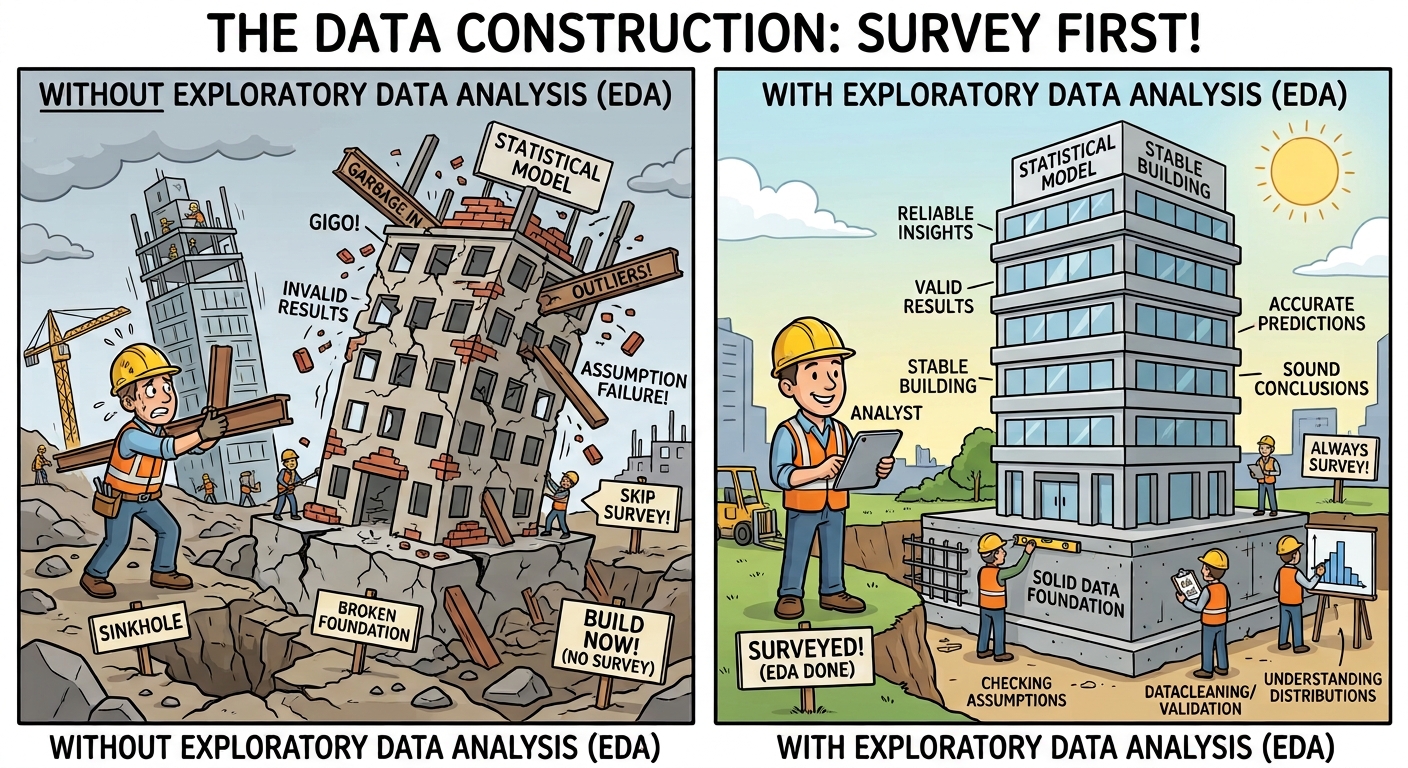
Nobody pours concrete without surveying the ground first. The same logic applies to everything we do this term — the model is only ever as sound as what it is built on.

Exploratory data analysis

Survey before you build in statistics is more formally known as exploratory data analysis - we’ll cover it in two weeks.

• This week — what have I actually got? What type is each variable, what shape does it take, where is its middle, how spread out is it, and what is odd or missing about it. All of it descriptive: statements about the data in front of us.
• Next week — what lies behind it? The probability distributions those shapes are drawn from, how to transform data that misbehaves, and the harder question of whether your data represents anything at all.

This week is deliberately the concrete one. Every single example comes from one real dataset, which we meet next.

Learning Objectives

By the end of this lecture you will:

1. Understand the four basic levels of measurement, and the finer statistical data types that build on them;
2. Be able to describe a variable — its shape, its middle, and its spread — and know when each summary is trustworthy;
3. Recognise missing values and outliers as information rather than nuisance;
4. Know the course dataset well enough to start asking questions of it.

Our dataset for the term

School performance in England, 2022/23

• Published every year by the Department for Education
• A full census of every school in England — not a sample
• Hundreds of variables on attainment, pupil characteristics and school characteristics
• We will use it in almost every week of this course Terminology
• GCSE - The exam everyone takes at age 16
• Ofsted - the Government Office for Standards in Education (quality assurance - they grade schools on how good they are)
• Academy - A type of state school outside of local authority control
• Maintained - A type of state school run by the local authority
• Attainment 8 and Progress 8 - Overall GCSE exam scores bundled together into a single exam performance metric

	Count
Schools with a KS4 result	4,631
Of which state-run	3,250
Variables in the full release	700+
Local authorities covered	153

What a row actually looks like

School	Type	Ofsted	Pupils	Attainment 8	% disadvantaged
King’s School	Academy	Good	789	54.3	16
Portslade Aldridge Community Academy	Academy	Good	953	44.8	26
Brighton Aldridge Community Academy	Academy	Requires improvement	838	36.2	45

• Every row is a school. Remember that — it matters later.
• We are never looking at individual pupils in this dataset.

Stress the unit of observation. Almost every mistake students make with this data comes from forgetting that a row is a school, not a child.

Attainment 8 — our main outcome variable

• Sums each pupil’s grades across 8 GCSEs
• Maths counted twice, English often twice
• Maximum possible score is 90; 40 is roughly a “standard pass” average
• Averaged across all Year 11 pupils to give a school-level score

It is a raw score. It takes no account of who a school admits — which is exactly the problem we spend weeks 6 to 8 solving.

Data types

Four levels of measurements

	Nominal	Ordinal	Interval	Ratio
Categorizes and labels variables	✔	✔	✔	✔
Ranks categories in order		✔	✔	✔
Has known, equal intervals			✔	✔
Has a true or meaningful zero				✔

• Developed by psychologist Stanley Smith Stevens (1906 - 1973)

• This is the classic starting point, and it is where most courses stop.
• We will start with this - but extend it later

Nominal

• Differentiates items based only on names; no order between them
• Also called categorical data
• What can be said about them?
  • ✅Equality: an Academy is not a Special school
  • ✅Mode: the most common category

In our data: school type, religious character, region, admissions policy.

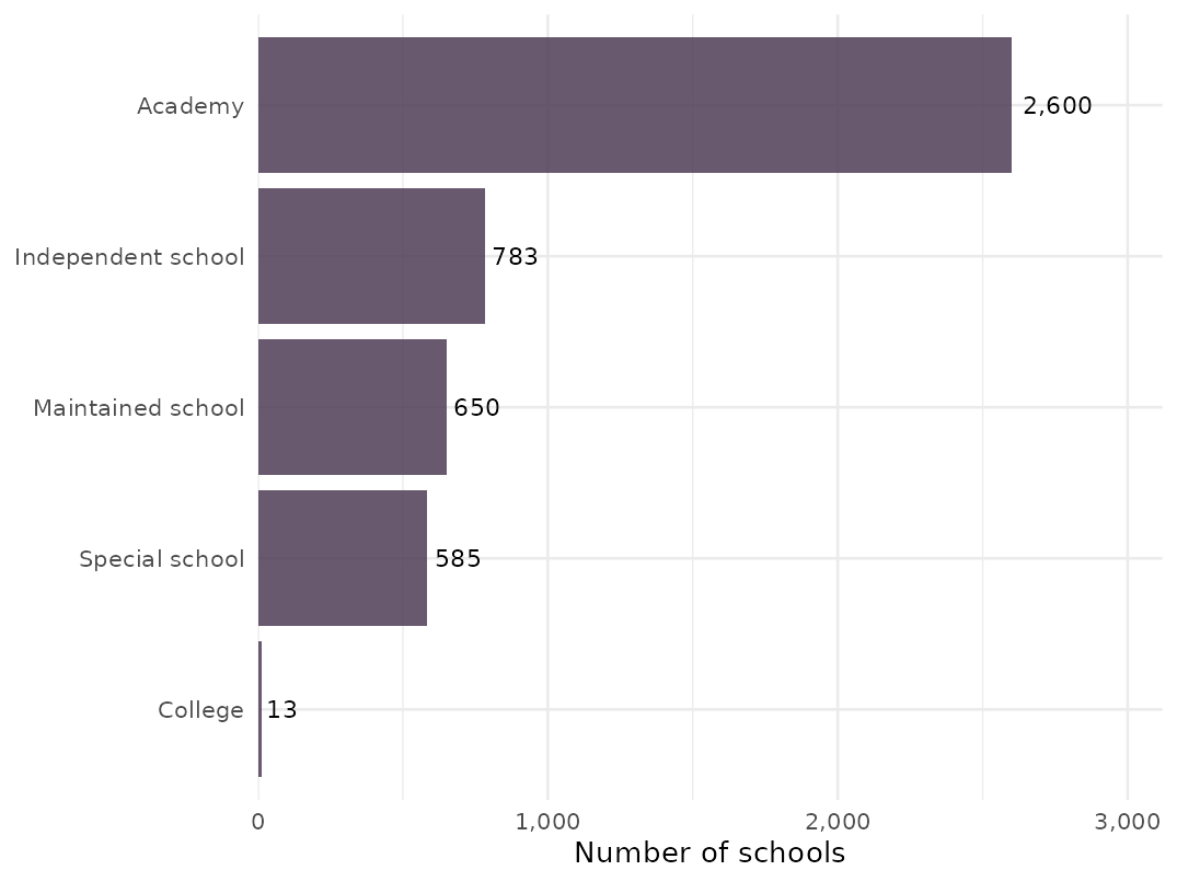
The bars can be reordered freely — there is no natural order here

Ordinal

• Allow for rank order, but not the relative degree of difference
• What can be said about them?
  • ✅ Equality; mode
  • ✅ Median: middle-ranked item
  • ❌ Differences between two levels; arithmetic mean
• Ordinal can be sub-divided into weak (Amazon star ratings on a product) and strong (1st, 2nd, 3rd finisher in a race)

In our data: Ofsted rating.

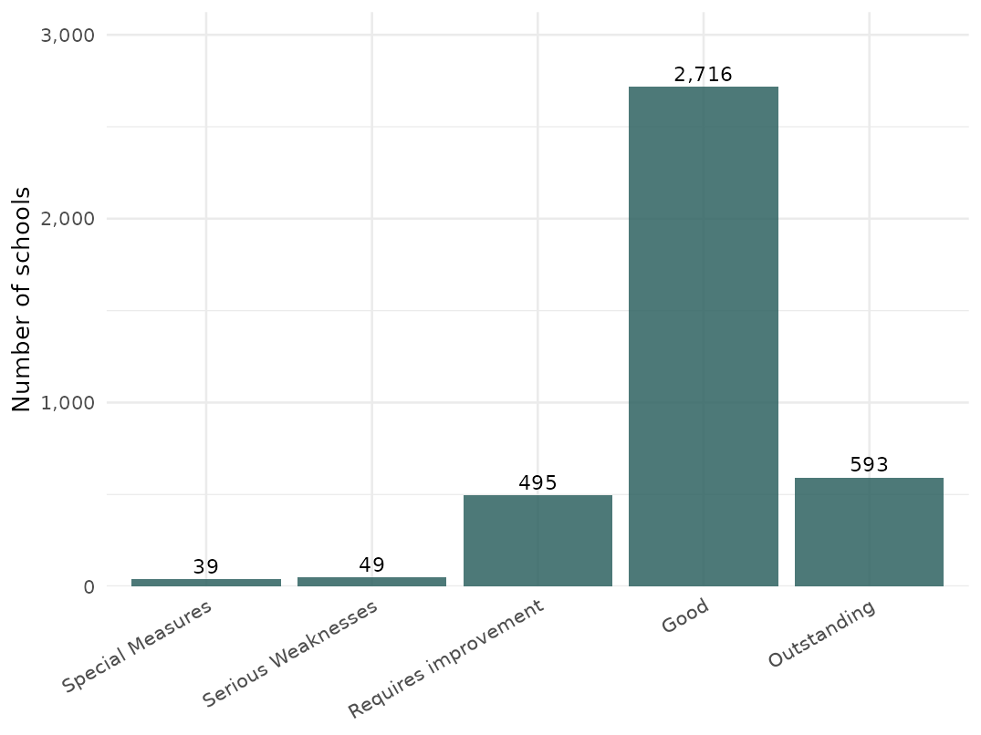
The order cannot be shuffled — but is Good → Outstanding the same size a step as Requires improvement → Good?

Interval and ratio

Interval — differences are meaningful, but the zero is arbitrary

• 100°C is not twice as hot as 50°C
• In our data: the date of the last Ofsted inspection. 2015 → 2018 is the same gap as 2018 → 2021, but “year zero” is a convention.

Ratio — a true, non-arbitrary zero, so ratios are meaningful

• ✅ Equality, mode, median, arithmetic mean, and ratio
• In our data: pupils on roll, Attainment 8, % disadvantaged. A school with 1,200 pupils really does have twice as many as one with 600.

Confusing Ratios: Progress 8

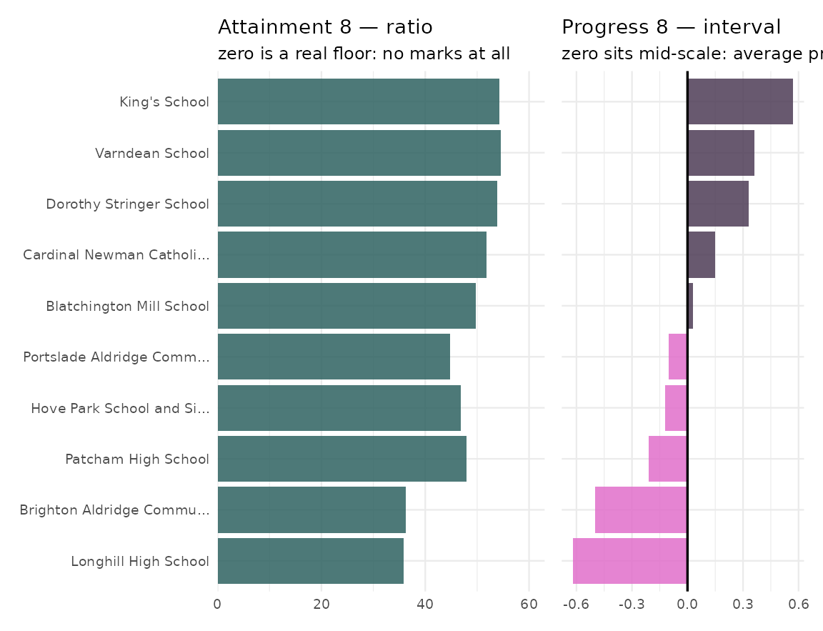
Progress 8 compares the progress pupils made with similar pupils nationally, each year.

• Zero means “average expected progress” - sits in the middle
• Positive is more, negative is less The zero is meaningful. So is it ratio data? No.
• King’s scores 0.57 and Blatchington Mill 0.03 — a ratio of 19:1.
• Not 19 times the progress!
• And Longhill is negative, so no ratio is possible at all.

Same ten Brighton schools on both panels. Left: bars start at a true zero, so “school A has 1.1 times the attainment of school B” is a sensible sentence. Right: bars straddle zero, so the same sentence is meaningless.

This is the slide that stops students assuming “has a zero” means “ratio”. P8MEA appears again later under real-valued additive, where its symmetry rather than its zero is the point.

Data types - extended

Simple statistical data types

Data type	Possible values	Level of measurement	Common distributions	Common model
binary	0, 1	nominal	Bernoulli	logistic, probit
categorical	“name1” … “nameK”	nominal	categorical	multinomial logit / probit
ordinal	ordered categories	ordinal	categorical	ordered logit / probit
binomial	0, 1, …, N	interval	binomial, beta-binomial	binomial regression
real-valued additive	any real number	interval	normal — symmetric	standard linear regression
count	0, 1, 2, …	ratio	Poisson, negative binomial	Poisson / neg. binomial regression
real-valued multiplicative	positive real	ratio	log-normal, gamma, exponential — skewed	GLM with a logarithmic link

Adapted from Statistical data type, Wikipedia (CC BY-SA)

The two columns worth dwelling on are the last two. The whole point of this table is that the data type determines the distribution, and the distribution determines the model. Everything in weeks 5 to 10 is an instance of this.

Every one of these is in our dataset

Data type	Variable	What it is
binary	single sex / mixed	Is the school single sex?
categorical	MINORGROUP	School type
ordinal	OFSTEDRATING	Ofsted rating
binomial	TFSM6CLA1A out of TPUP	Disadvantaged pupils out of the cohort
real-valued additive	P8MEA	Progress 8
count	TOTPUPS	Pupils on roll
real-valued multiplicative	PERCTOT	% of sessions missed

• Bea will explain more about distributions next week
• And We will meet the model in the right-hand column of the previous slide for almost all of these before the course ends.

And your computer will represent them too

Statistical type	Programming type	In R	In Python / pandas
real-valued (interval or ratio)	floating point	numeric / double	float64
count	integer	integer	int64
binary	Boolean	logical	bool
categorical	enumerated type	factor	category
ordinal	ordered enumerated type	ordered factor	Categorical(ordered=True)
random vector	list or array	vector	ndarray / Series
random matrix	two-dimensional array	matrix	2-D ndarray

Left two columns adapted from Statistical data type, Wikipedia (CC BY-SA)

A Data Encoding Warning

• Ofsted rating is ORDINAL
• If we store it as {Special Measures:1, …, Outstanding:5}, is it ORDINAL, or INTERVAL?

school_id	region	ofsted	parent_survey	attainment8
101248	3	4	5	51.2
101319	7	2	3	43.8
101422	1	5	5	58.6
101507	3	1	2	37.1
101663	9	3	4	46.9

region is a nominal code. ofsted and parent_survey are ordinal codes. school_id is a label. Only attainment8 is a measurement.

Five numeric columns. One number.

Still ordinal. Storing something as a number does not make the gaps equal — and nothing in the file will tell you which is which.

…and this is a common analysis error

• Categorical or ordinal data often arrives already coded as numbers
• Software cannot tell. read_csv sees 1, 2, 3, 4, 5 and hands you a numeric column
• Nothing errors. Every summary works. Every model runs.
• So people put it into a regression as a continuous predictor and report “each additional unit of Ofsted is worth x points”

Descriptive statistics: the middle and the spread

Key metrics

Attainment 8 across all English schools

Schools (n)	Mean	Median	Std. dev.	Minimum	Maximum
4,631	39.8	43.6	17.5	0.0	87.6

• Finding the size, edges and middle of the data gives us a rough sense of what we are dealing with and can be a useful short-hand. An important first step.

• Quantity (count)
• The middle (mean, median, mode)
• The spread (minximum, maximum, standard deviation)

• Mean — add everything up, divide by how many
• Median — line them all up, take the middle one
• Mode — the most common value

• However, in data analysis terms, this would be the statistical equivalent of preparing some food by only looking at your shopping list of ingredients!

Descriptive statistics - Visualisation

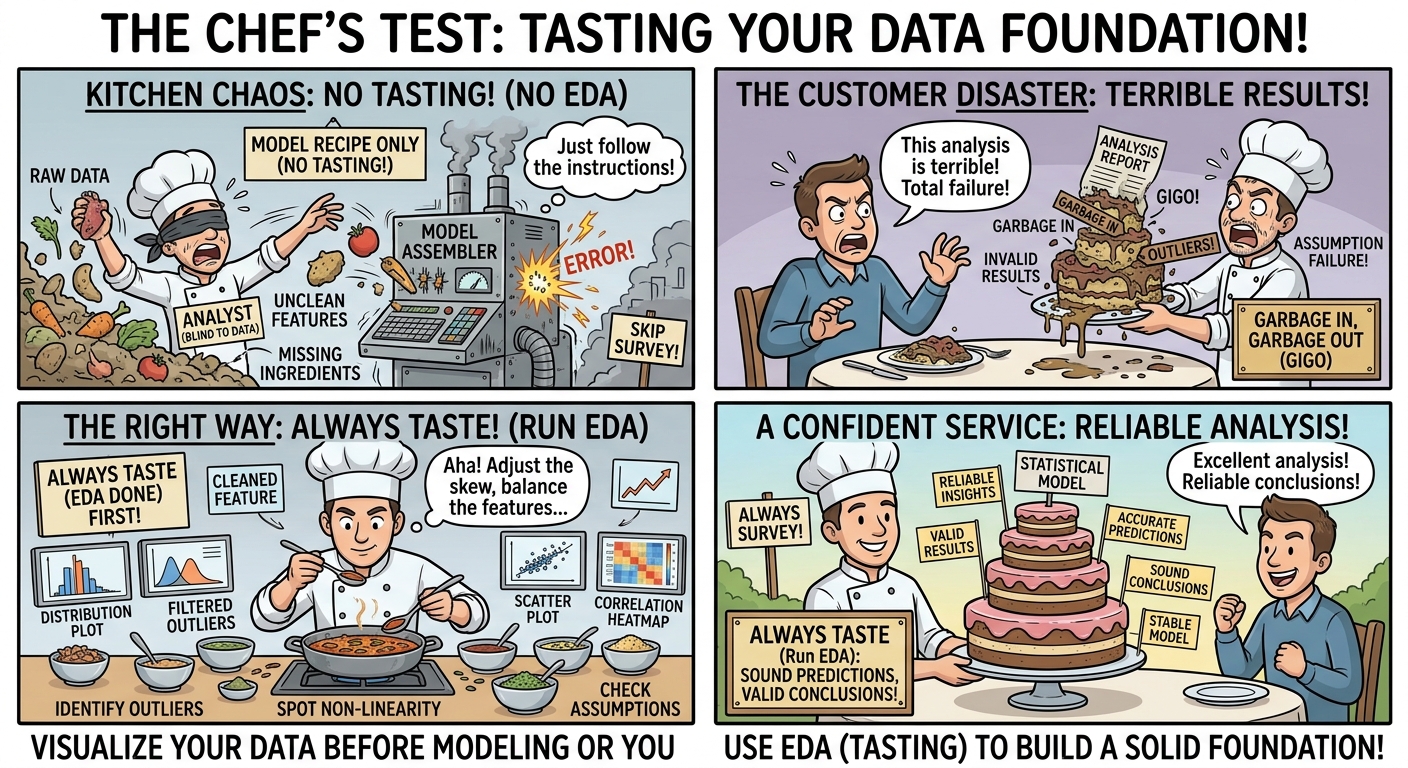
Visualising Your Data - Frequency Distributions

A frequency distribution lets you see the full shape of your data - and all of it’s quirks.

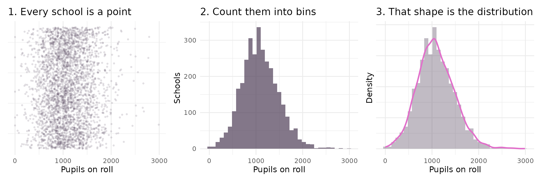
• The histogram is the workhorse: bin the values (any size bin you like), count how many land in each bin
• The smooth curve is the same information with the bins taken away - More Next week
• Almost everything else in this course starts by asking what shape (Frequency Distribution) a variable has

A boxplot is a summarised histogram

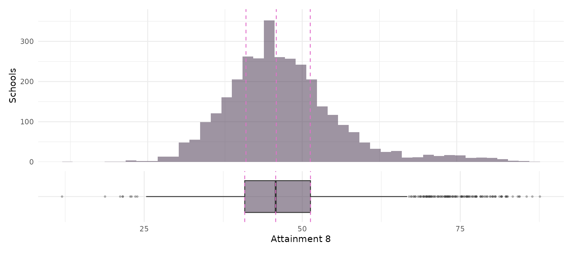
• A boxplot or a box and whisker plot - same data, same axis. The dashed lines are the quartiles
• The box holds the middle 50% of schools (the inter-quartile range or IQR); the line inside it is the median
• The whiskers reach the furthest point within 1.5 × the box width; anything beyond it (the dots) are known as outliers - more later
• A boxplot is a histogram with the shape thrown away and five numbers kept

Which is the trade. You lose the shape entirely - a boxplot cannot show you two humps - but you gain the ability to put many of them side by side, which we do later in this lecture.

Four ways to draw the same distribution

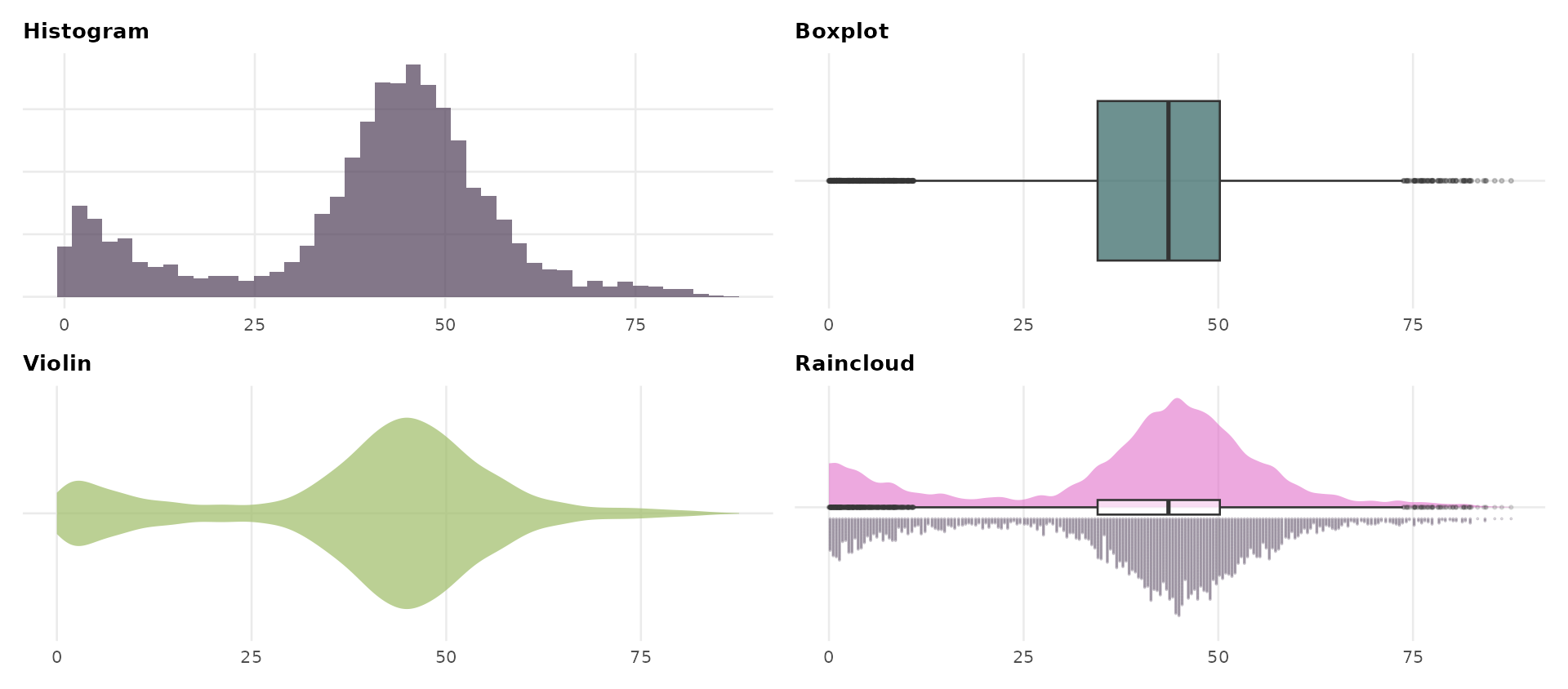
The same 4,631 schools and the same Attainment 8 scores, four times over. Three of these show you that the data has more than one hump. One of them does not.

What each one keeps, and what it throws away

	What it shows you	What it hides	Reach for it when
Histogram	the full shape, every bump and gap	no summary statistics marked	exploring one variable properly
Boxplot	median, quartiles, outliers — five numbers	the shape, completely	comparing many groups at once
Violin	the full shape, mirrored	individual points, and how many there are	comparing a few groups where shape matters
Raincloud	shape, summary and every observation	gets crowded fast	one or two groups, when you want to show everything

All four are answering the same question — how many observations fall where? They differ only in how much they summarise before they show you.

The boxplot on the last slide looked perfectly ordinary. The data it was drawn from has three separate humps — special schools, independent schools and mainstream schools, piled on top of each other. A boxplot will never tell you that. Always look at the shape before you summarise it.

The three humps are at roughly 2.5, 21 and 45 on the Attainment 8 scale, and they correspond to special schools, independent schools and mainstream schools respectively. Worth naming out loud - it connects straight back to the population-versus-sample slides earlier, where we filtered exactly these groups out.

If anyone asks why the violin looks symmetric: it is the same density drawn twice, mirrored. It carries no more information than half of it would.

Count Data

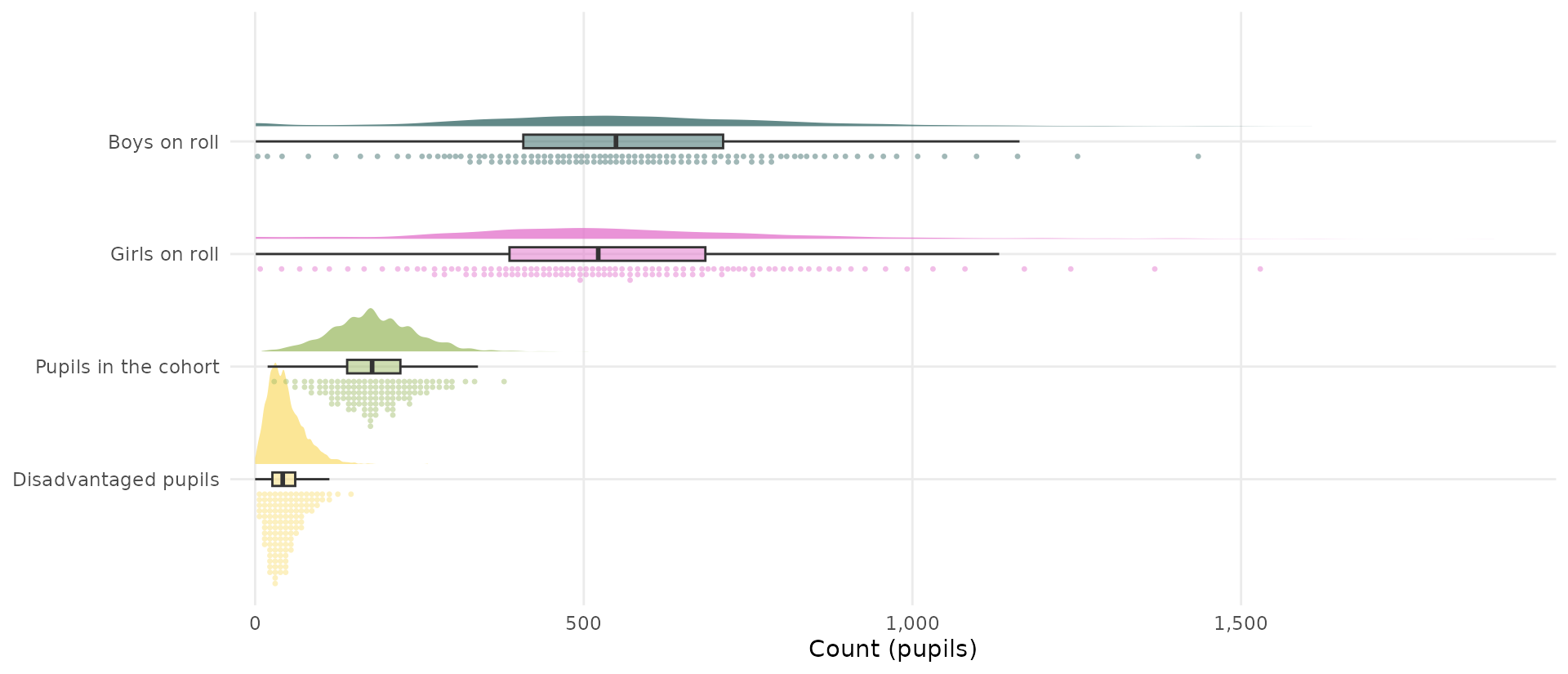
Five counts, one axis. Each cloud is the distribution, the box the quartiles, the rain below it the schools themselves.

Count Data

• Whole numbers, never negative, no upper limit in principle
• A mean of 1085 pupils is meaningful; a school with 1,204.7 pupils is not
• Distribution: Poisson or negative binomial, not normal

• Now look at the bottom of that chart
• Disadvantaged pupils (median 42) all but vanishes beside boys on roll (median 549)
• Same data type, same axis — and still not comparable

Hold that thought. Is a school with 120 disadvantaged pupils more unusual than one with 900 boys on roll? You cannot answer that from this chart — the units are different and so are the spreads. Later today we fix it, by converting both to standard scores.

Binomial Data

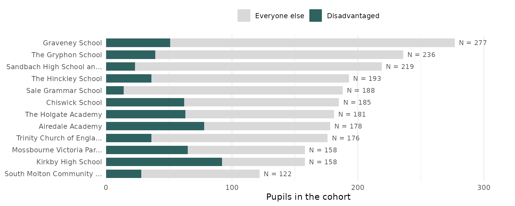
• A count bounded above by the size of the cohort — it cannot exceed an upper ceiling N — e.g. a finite number of coin tosses, or children in a school
• Each bar is a school’s ceiling. The teal part is the count; it can never spill past the end of its own bar
• Every school has a different ceiling, which is why the raw count tells you so little
• Distribution: binomial. This is why a percentage is the natural summary.

Real-valued additive

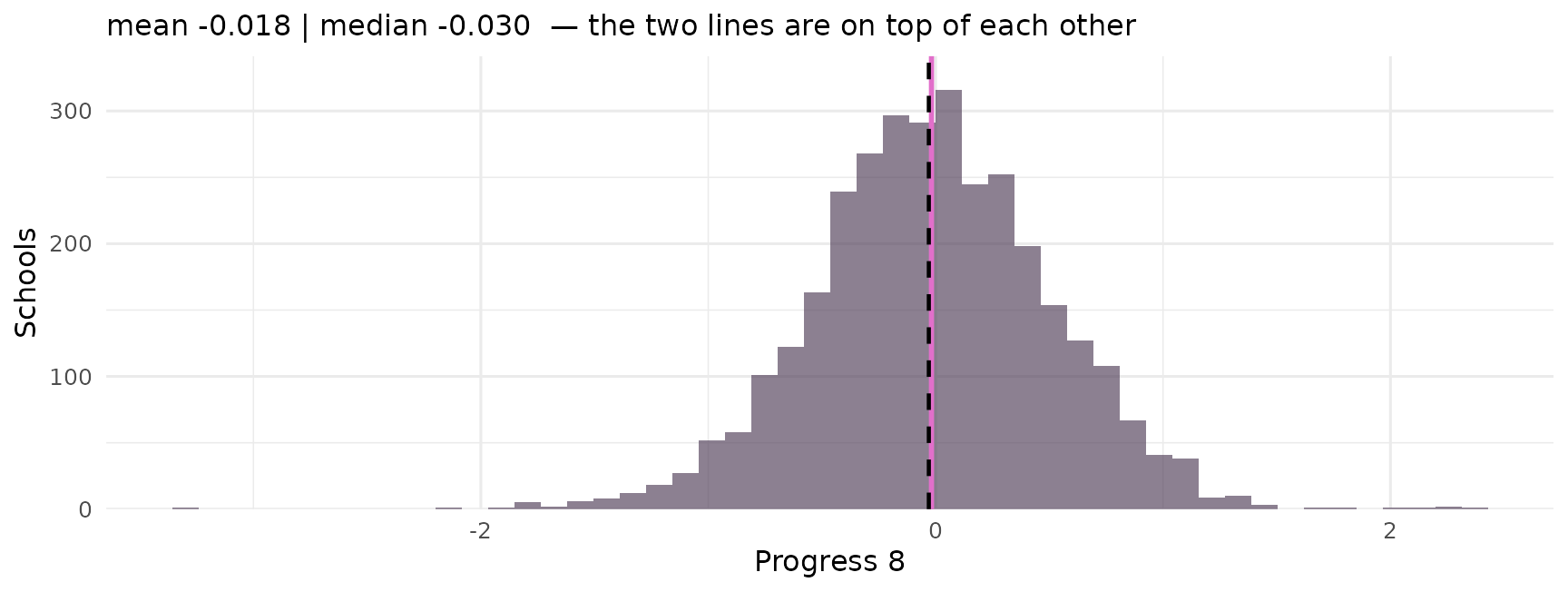
• A real number can be placed anywhere on a line - i.e. can have a decimal
• Can be negative. Symmetric about its mean.
• Mean -0.018 (pink like), median -0.030 (black dotted) — almost identical
• Distribution: normal. Model: ordinary linear regression — weeks 6 and 7.

Real-valued multiplicative

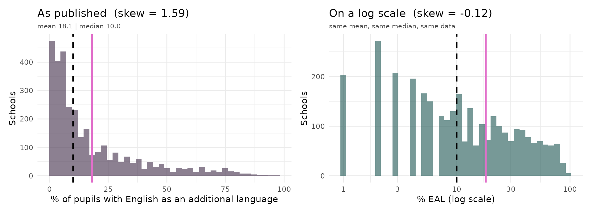
• Strictly positive, and strongly skewed (mean and median very different) — most schools have few EAL pupils, a long tail have very many
• Both panels show the same percentages, the same mean and the same median. Only the spacing of the axis changes: equal distances now mean equal multiples rather than equal amounts (additive)
• On that spacing the distribution is very nearly symmetric, and the mean sits close to the middle of it
• This is not a trick. It is what the data type tells us to do — and it is exactly what we do in week 6 when we fit a log-log model.

Real-valued multiplicative

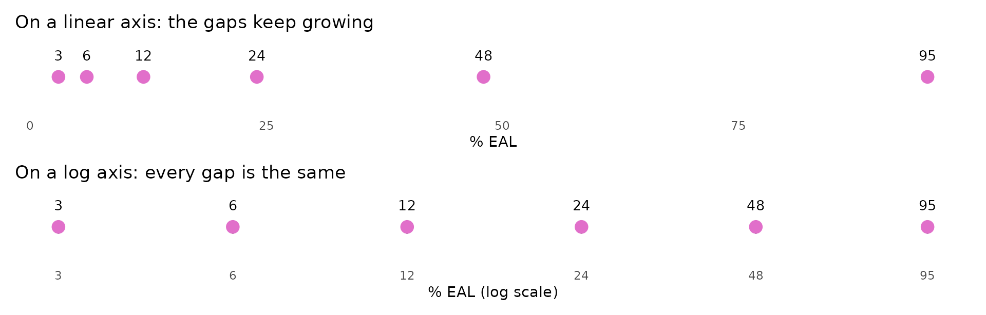
Six real schools, each with roughly twice the share of the one before. The jump from 3% to 6% and the jump from 48% to 96% are the same size — as multiples. A logarithmic axis is simply an axis that agrees.

Next week. Bea takes this apart properly — exponentials, logarithms, and when to reach for them. For now, just notice that changing the spacing changed the shape.

If someone asks: the pink line is the ordinary arithmetic mean of the percentages, plotted at the same value on both panels. The natural centre of a multiplicative variable is really the geometric mean - exp of the mean of the logs - which lands closer to the median. Not worth opening up here, but it is the reason logged models are quoted as percentage changes.

Why any of this matters

If your outcome is…	…the model you need is	Covered in
real-valued additive	linear regression	weeks 6, 7
real-valued multiplicative	linear regression on logged data	weeks 6, 7
grouped / nested	linear mixed effects	week 8
binary	logistic regression	week 8
ordinal	ordered logistic regression	week 8
count	Poisson regression	week 8

• Choosing the wrong one does not usually throw an error.
• It quietly gives you a plausible, wrong answer.
• Knowing your data type is the defence.

Attainment 8 across all English schools (again)

Schools (n)	Mean	Median	Std. dev.	Minimum	Maximum
4,631	39.8	43.6	17.5	0.0	87.6

• Quantity: 4,631 schools
• The middle: mean 39.8, median 43.6
• The mean is lower than the median. Why?

Do not resolve this yet — it is the hook for the visualisation section.

So why is the mean below the median?

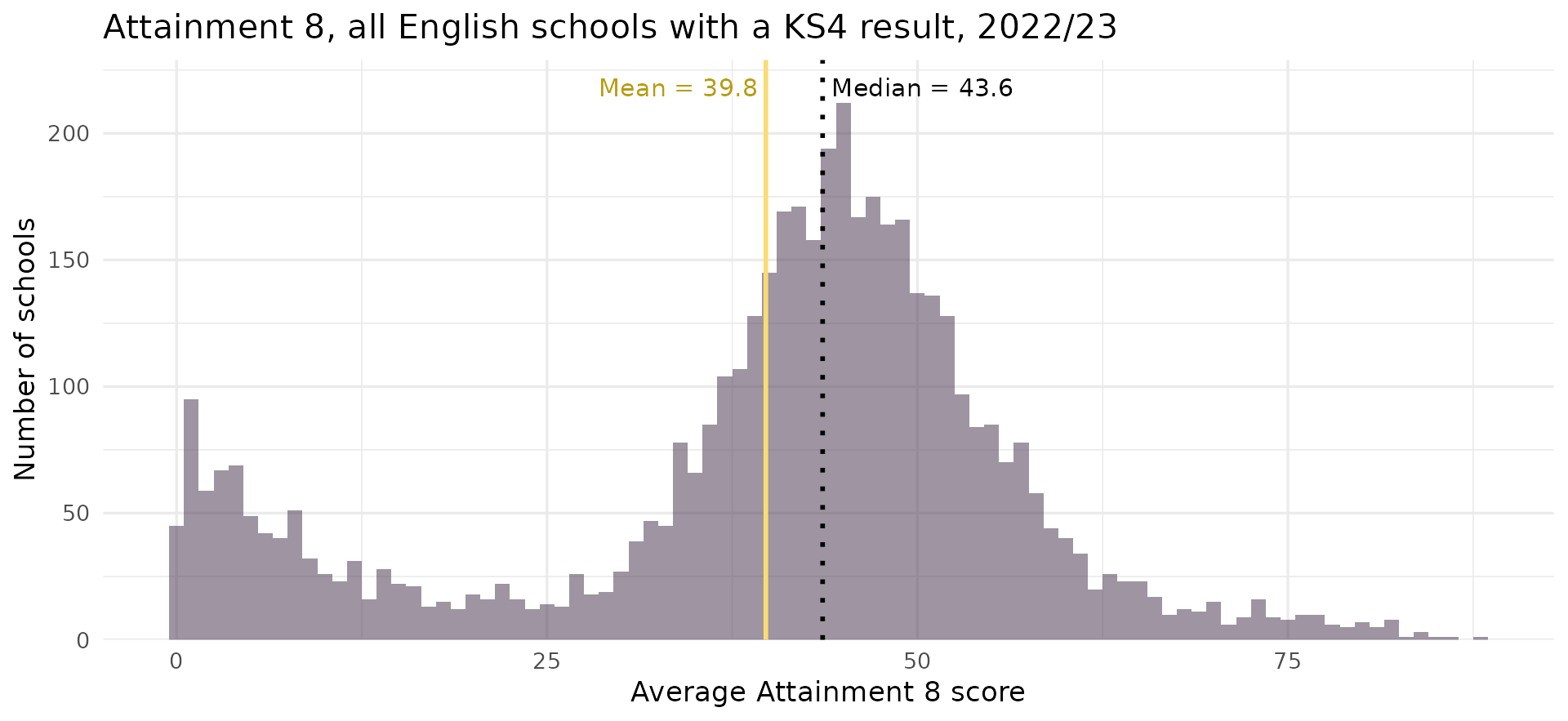
• One summary table told us mean < median. One picture tells us why.
• There is a whole second population of schools down at the left.

The same data, split by school type

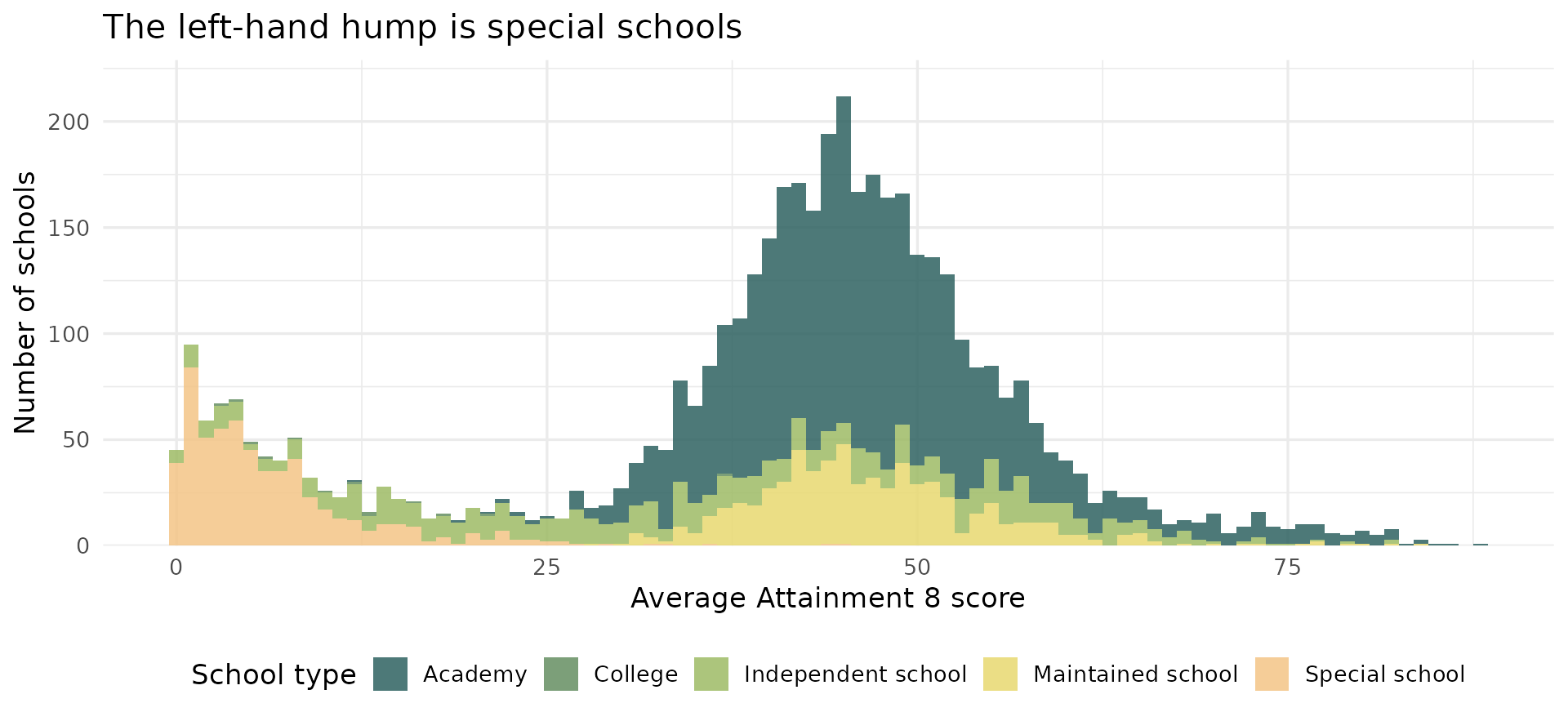
• Special schools educate pupils with significant special educational needs
• Attainment 8 was never designed to compare them with mainstream schools

What that does to the headline number

School type	n	Mean	Median	Std dev
Special school	585	6.5	4.7	6.3
College	13	12.7	12.2	9.1
Independent school	783	35.6	35.9	18.9
Academy	2600	46.9	45.8	9.7
Maintained school	650	46.9	45.8	7.9

• Mixing these together produces a mean that describes no real school
• The fix is not statistical, it is knowing what is in your data
• From week 6 onwards we work with mainstream secondaries only — now you know why

Careful — we have just changed what we are studying

	School type	Schools
Dropped	Independent school	783
Dropped	Special school	585
Dropped	College	13
Kept	Academy	2,600
Kept	Maintained school	650

• We began with a population: every school in England with a KS4 result
• Filtering to academies and maintained schools leaves a subset — or a sample and it is not a random one
• Anything we now conclude is about mainstream state-funded secondaries, not “schools”

Dropping cases is a decision, not a technicality

• Special schools are excluded because Attainment 8 was never designed to describe them — defensible, but it removes the lowest-attaining pupils in the country from view
• Independent schools are excluded because they sit outside the state system — also defensible, and it removes much of the top of the distribution
• Neither group left by accident. We chose.

Recall the first slides: a sample only tells you about the population it was drawn from. The moment you filter, you have redefined that population — so say which one you mean.

Next week. Representative data, selection bias, and what happens to your conclusions when the cases you dropped are not like the ones you kept.

Worth saying out loud that this is the single most common unexamined step in student analyses: a filter applied early, for a good reason, and then never mentioned again in the write-up.

The assessment asks them to justify their data choices — this is what that means in practice.

The middle is not enough

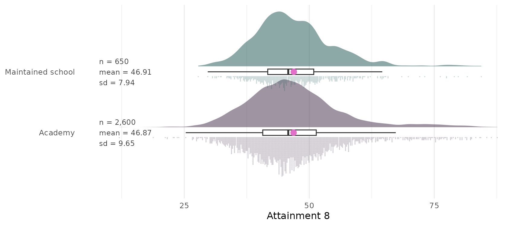
• The two means differ by 0.04 of a point — for practical purposes, identical
• The spread does not: academies are noticeably wider (more rain) - larger variance
• Report only the mean and these two look like the same story. They are not.

Variance and standard deviation

Variance is the average squared distance from the mean: \[\sigma^2 = \frac{\sum_{i=1}^{n} (y_i - \bar{y})^2}{n}\] \(y_i\) = value for any given school in our dataset

\(\bar{y}\) = the average value across all schools

Standard deviation is its square root: \[\sigma = \sqrt{\sigma^2}\]

• Squaring is what makes variance awkward to talk about:
• if \(y\) is in GCSE points, the variance is in points².
• The standard deviation is back in the original unit (GCSE points in this case), which is why we almost always report that instead.

School type	Mean	Variance	Std dev
Academy	46.87	93	9.65
Maintained school	46.91	63	7.94

Same mean. The variance of academy scores is close to half again as large.

Squaring also means outliers count heavily — a school 30 points from the mean contributes 900, not 30.

Spread across all four school types

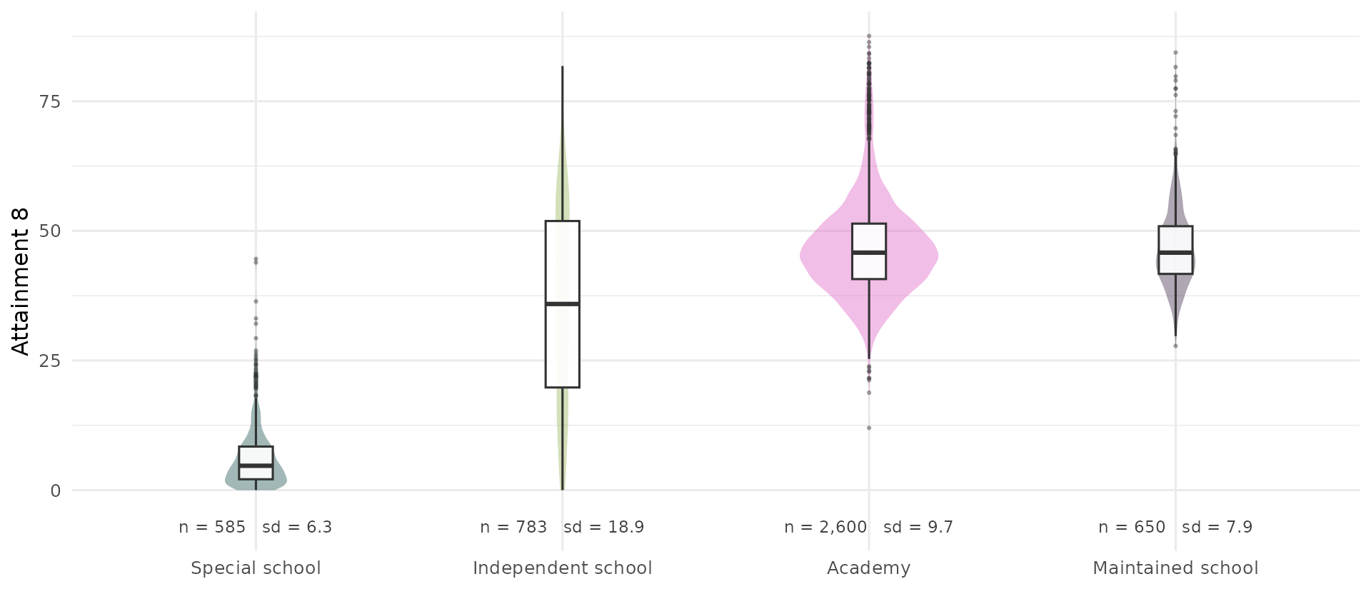
• The box gives you the median, the quartiles and the outliers
• The width of the violin is proportional to how many schools are in that group — a boxplot alone would hide that
• Independent schools: widest spread by far (sd 18.9), and the only group where the box spans more than 30 points

When is the mean a good summary?

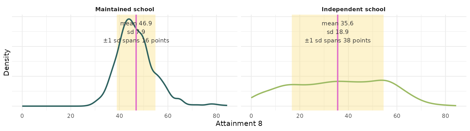
• Mean a better summary when variance is small and distribution normal
• If the data are roughly normal, about two thirds of observations sit inside the shaded band
• For maintained schools that band is ~16 points wide — the mean tells you a lot
• For independent schools it is ~38 points — more than a third of the whole 0–90 scale
• Same statistic. Very different amount of information.

We are borrowing something here. “Roughly normal” and “about two thirds” are properties of a specific distribution that we have not defined. Next week Bea makes both precise — for now, take the two-thirds rule on trust and notice what it buys you.

A mean without a spread is half a number

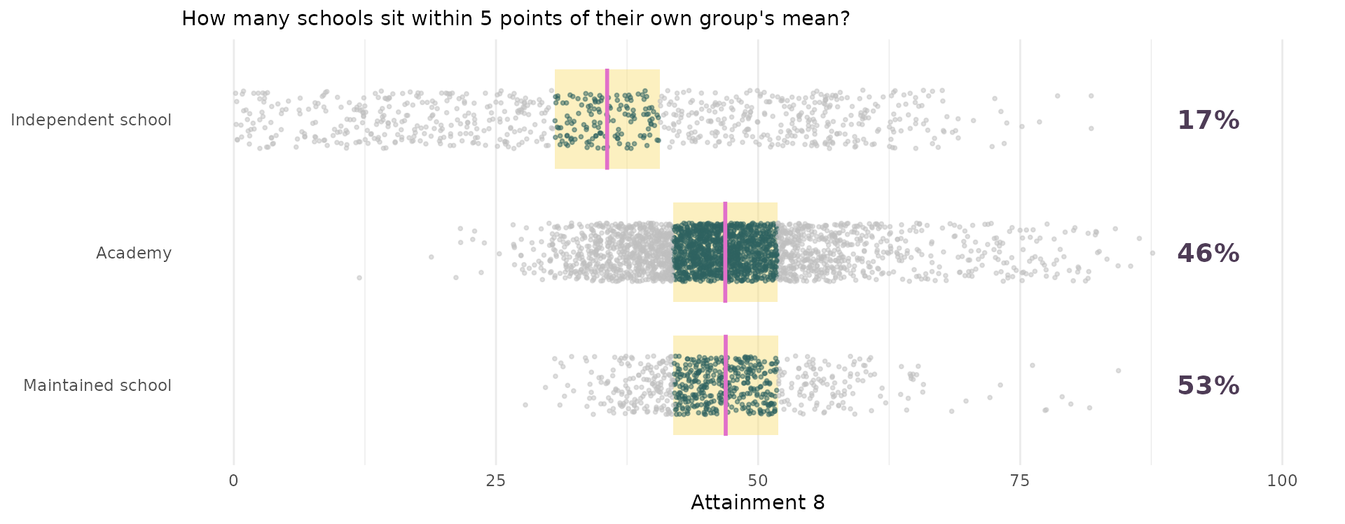
• Same window, same width, three very different answers
• A large standard deviation means individual cases sit far from the mean, so the mean describes no one in particular — for independent schools it speaks for fewer than one school in five
• A small standard deviation means the mean is a good stand-in for a typical case
• This is why you should never report a mean on its own

The caveat to state out loud: the two-thirds rule assumes roughly normal data. For the skewed variables we saw earlier the mean is a questionable choice in the first place, which is why we looked at the shape before computing anything.

Counts, rates and the denominator

A count answers “how many?” — and mostly tells you how big the place is.

A rate divides that count by something that makes it comparable:

\[\text{rate} = \frac{\text{numerator}}{\text{denominator}}\]

• The numerator is what you are counting — disadvantaged pupils in a school
• The denominator is what you are counting it out of — all pupils in that school’s cohort
• Our data ships both: TFSM6CLA1A is the count, TPUP is the denominator, and PTFSM6CLA1A is the rate they produce

Choosing the denominator is a decision about what you mean, not an administrative detail. Per pupil, per school, per head of population and per square kilometre answer different questions.

Big schools have big numbers

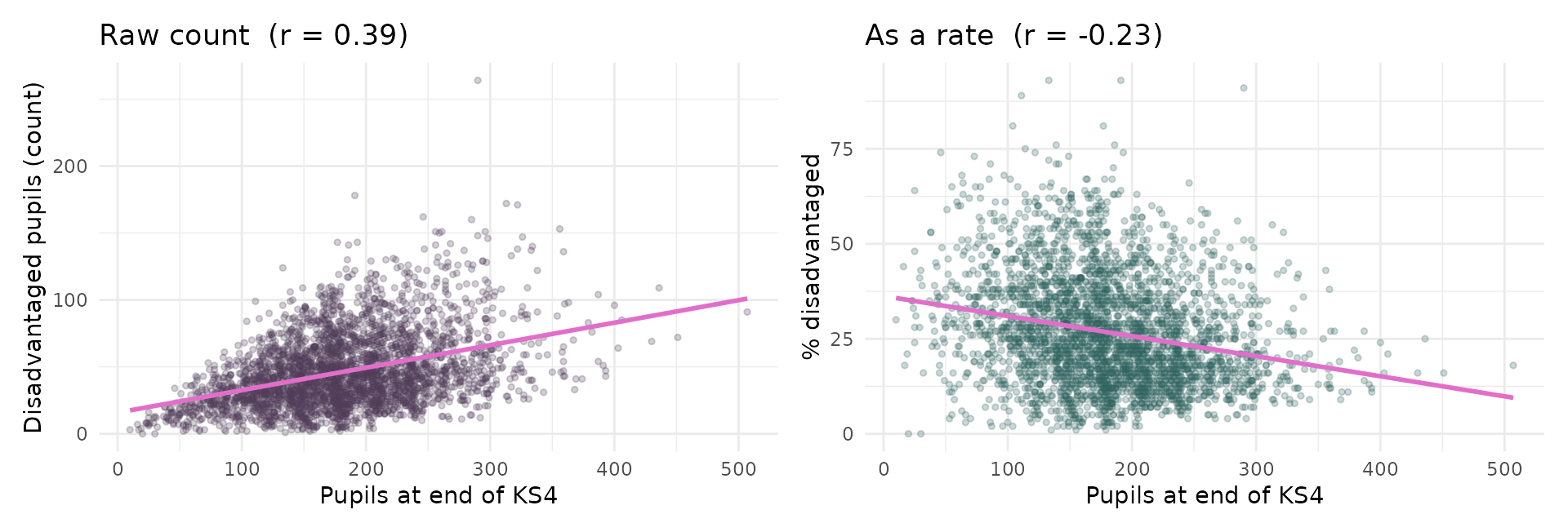
• The left panel is a strong relationship that tells you nothing: big schools have more of everything
• The right panel divides by size, and the relationship all but vanishes
• Raw counts mostly measure how big a place is. Almost always, you want a rate.
• A rate removes the effect of size. It does not make different variables comparable with each other — a percentage and a head-count still live on different scales. That needs one more step.

The most common mistake in student data journalism. One slide is enough to inoculate against it, and it pays off again in week 6.

Comparing things measured on different scales

Variable	Mean	Std dev
Attainment 8	46.9	9.3
% sessions missed	9.2	2.6
% disadvantaged	26.7	14.4
% low prior attainment	22.2	10.0
Pupils on roll	1085.2	397.7

A school is 3 points above average on Attainment 8 and 300 pupils above average in size. Which is the more unusual? On the raw numbers the question is meaningless — the units are different.

The standard score (z-score)

\[z = \frac{x - \bar{x}}{\sigma}\]

Subtract the mean, divide by the standard deviation.

• The result is measured in standard deviations, so every variable lands on the same scale
• \(z = 0\) is exactly average, \(z = +1\) is one standard deviation above, and the sign gives the direction
• After standardising, every variable has mean 0 and standard deviation 1

Weeks 9 and 10 standardise every variable before PCA and clustering — otherwise “pupils on roll”, with a standard deviation of 398, would drown out “% sessions missed”, with a standard deviation of 2.6.

One school, five variables

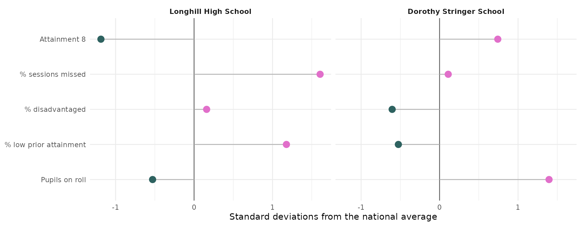
• Five variables, five different units, one readable picture
• Two schools three miles apart in Brighton, with mirror-image profiles
• Longhill sits well above average on absence and below it on attainment — while its disadvantage is only just above average
• That contrast is the question weeks 6 to 8 spend three weeks answering

Special values: null and outliers

Null values

• Representing the absence of data or an unknown value
• Different from zero or a blank space
• Null values should be excluded before computing mean or std

The DfE does not leave blanks — it publishes codes:

Code	Meaning
SUPP	Suppressed, because the number of pupils is too small to publish safely
NP	Not published
NE	No entries
LOWCOV	Low coverage — too few pupils for a reliable figure
NEW	School too new to have results

SUPP is disclosure control, not an error. A missing value here tells you the school is small — which is information, and it is not missing at random.

This is the single most useful practical thing in the lecture. It is also exactly what the na_values list in the practicals is doing.

How much is missing?

Variable	Missing
Attainment 8	0.0%
Progress 8	21.9%
Pupils on roll	0.3%
% disadvantaged	21.9%
Ofsted rating	16.0%
Overall absence	22.0%

• Always check this before you compute anything
• And ask why each one is missing, not just how many

Missing values have a distribution too

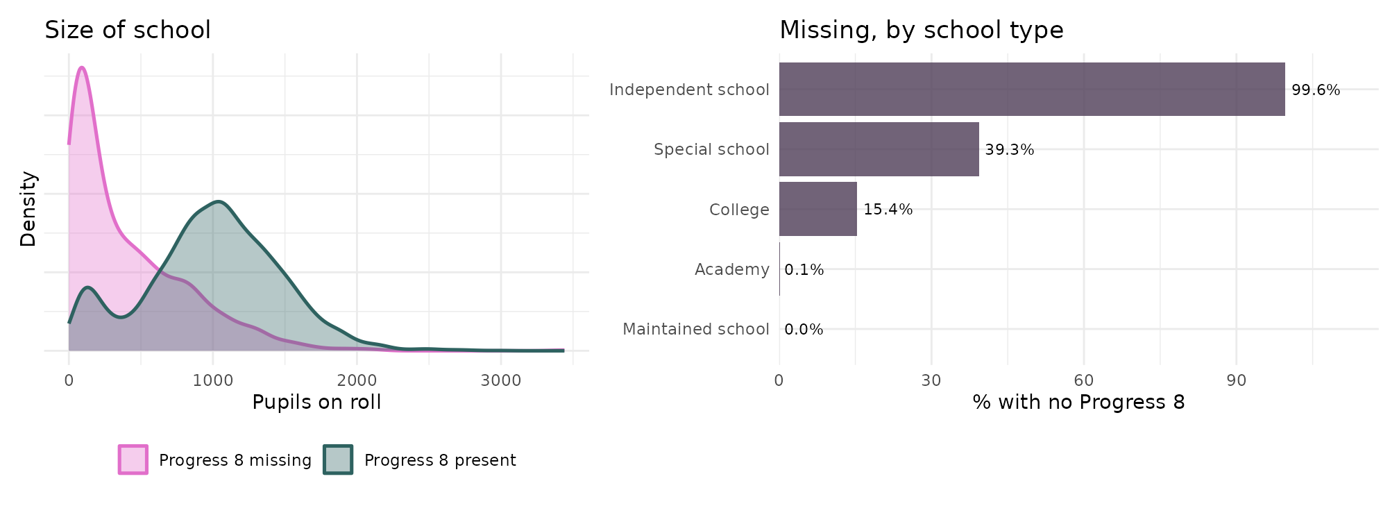
• If values went missing at random, the two curves on the left would sit on top of each other
• Median size where Progress 8 is missing: 247 pupils. Where it is present: 1,019
• Independent schools are missing it 99.6% of the time; maintained schools 0.0%

So the gaps are data

• SUPP means suppressed because the numbers are small — so a gap is telling you the school is small
• Independent schools sit outside the state accountability system, so a gap can also mean “not measured here”
• Drop every incomplete row and you have quietly deleted small schools and independent schools from your analysis
• Which is a decision, exactly like the filtering we did earlier

Always look at which cases are missing before you decide what to do about them.

This is the replacement for the Null Island slide. The point is stronger with our own data: missingness here is structured, predictable, and informative, rather than being an absence of information.

Ties directly back to the population-to-sample slides, and forward to next week’s treatment of representativeness.

Outliers

• A data point that differs significantly from other observations
• There are three types of outliers
• Please explain the rationale for removing any identified outliers, including the criteria and methods used

Type	Source	Handling
Error Outliers	Mistakes in collection, entry or measurement — e.g. a temperature sensor reading 500 °C	Should be corrected or removed
Irregular Pattern Outliers	Genuinely occur, but do not follow the general pattern — e.g. a spike in sales on Black Friday	May indicate events worth investigating. If studying the overall pattern, remove
Influential Outliers	Appear extreme but are integral to the underlying pattern — e.g. a special school in our attainment data	Keep them; removing them distorts the analysis or hides something important

Previously this was three near-identical slides revealing one row at a time. Consolidated. If you want the reveal back, wrap each row in a fragment.

What counts as an outlier?

Two standard rules, and they are just conventions:

The standard score

Use the \(z\) we met earlier, and flag anything with \(|z| > 3\) — or 2, or 2.5, depending on who you ask.

\(z\) measures how far from average a value is. The threshold is what turns that into a claim about outliers.

Tukey’s fences

Flag anything below \(Q_1 - 1.5 \times IQR\) or above \(Q_3 + 1.5 \times IQR\).

Widen to \(3 \times IQR\) for “far out” values.

Rule	Schools flagged	% of schools
|z| > 2	165	5.1%
|z| > 3	62	1.9%
Tukey 1.5 x IQR	136	4.2%
Tukey 3 x IQR	7	0.2%

Four rules, four answers, on the same 3,250 schools. “Outlier” is a choice, not a fact — so say which rule you used.

Error, or the most interesting thing in your data?

School	Local authority	Attainment 8	z
The Henrietta Barnett School	Barnet	87.6	+4.36
Wilson’s School	Sutton	86.4	+4.23
Queen Elizabeth’s School, Barnet	Barnet	85.5	+4.14
St Olave’s and St Saviour’s Grammar School	Bromley	84.4	+4.02
Kendrick School	Reading	84.3	+4.01

• 62 schools are beyond 3 standard deviations, and almost all of them are at the top
• Every school in that table is a selective grammar school
• These are not data errors. They are the single most informative cases in the file

Delete your outliers and you would have deleted the evidence that selection matters enormously — which is exactly the question weeks 6 to 8 are about.

This is the point to labour. An outlier is a case that does not fit the pattern you assumed. Sometimes that means the measurement is wrong. Just as often it means the assumption is wrong, and the case is the finding.

Contrast with the low end: Stephenson Studio School at 12.0 is a studio school with a tiny cohort, which is closer to the “different kind of thing” category we saw with special schools.

Tukey’s fences on our data

Dataset	Lower fence	Upper fence	Flagged as outliers
All schools	10.9	73.8	660
Mainstream secondaries only	25.3	66.9	136

• On the full dataset almost nothing is flagged — the special schools have stretched the quartiles so far that the fences swallow them
• On mainstream secondaries the method starts behaving sensibly
• A rule applied to the wrong population gives a confidently wrong answer

Overview

Exploratory data analysis, part 1 — what have we got?

• Our dataset for the term — DfE school performance, 2022/23
• Data types — Stevens’ four levels, and the finer statistical types that tell you which distribution and which model
• Descriptive statistics: shape — what a distribution is, and how to read a histogram and a boxplot
• Descriptive statistics: middle and spread — why the mean sat below the median, and why a mean without a standard deviation is half a number
• Making things comparable — counts, rates and standard scores
• Special values — DfE suppression codes, missingness that is not random, and outliers

Next week

Everything today was descriptive — statements about the 3,000-odd schools actually in front of us. Next week Bea turns that around.

• We kept saying things like “counts are Poisson” and “roughly normal, so about two thirds”. Next week those become real objects with parameters you can compute with, rather than labels
• We put absence on a logarithmic axis and watched it turn symmetric. Next week: why that works, and when to do it
• We filtered out special and independent schools and watched the headline number move. That was us changing the population on purpose. Next week: the bias that was already there before you touched anything

Same two weeks, same question — can I trust what this data seems to be telling me?

Practical

You will do all of that again yourself, on the same data, slicing it a different way.

• Every step is given in both R and Python — pick whichever you prefer
• Read and join the three DfE files, and handle the suppression codes properly
• Classify the variables, then describe and plot one of them
• Choose your own grouping variable — Ofsted rating, gender, religious character, local authority — and compare across its groups
• Find what is missing, work out whether it is missing at random, and flag the outliers
• Finish by writing down what your data can and cannot support a claim about

Bring questions. The last task is the one the rest of this course exists to answer.